library(tidyverse)
library(gapminder)

p <- ggplot(data = gapminder,
            mapping = aes(x = gdpPercap,
                          y = lifeExp))


p + geom_point()01 — Sociol 232: Visualizing Social Data
January 23, 2024


Get up and Running: Install R

Install RStudio
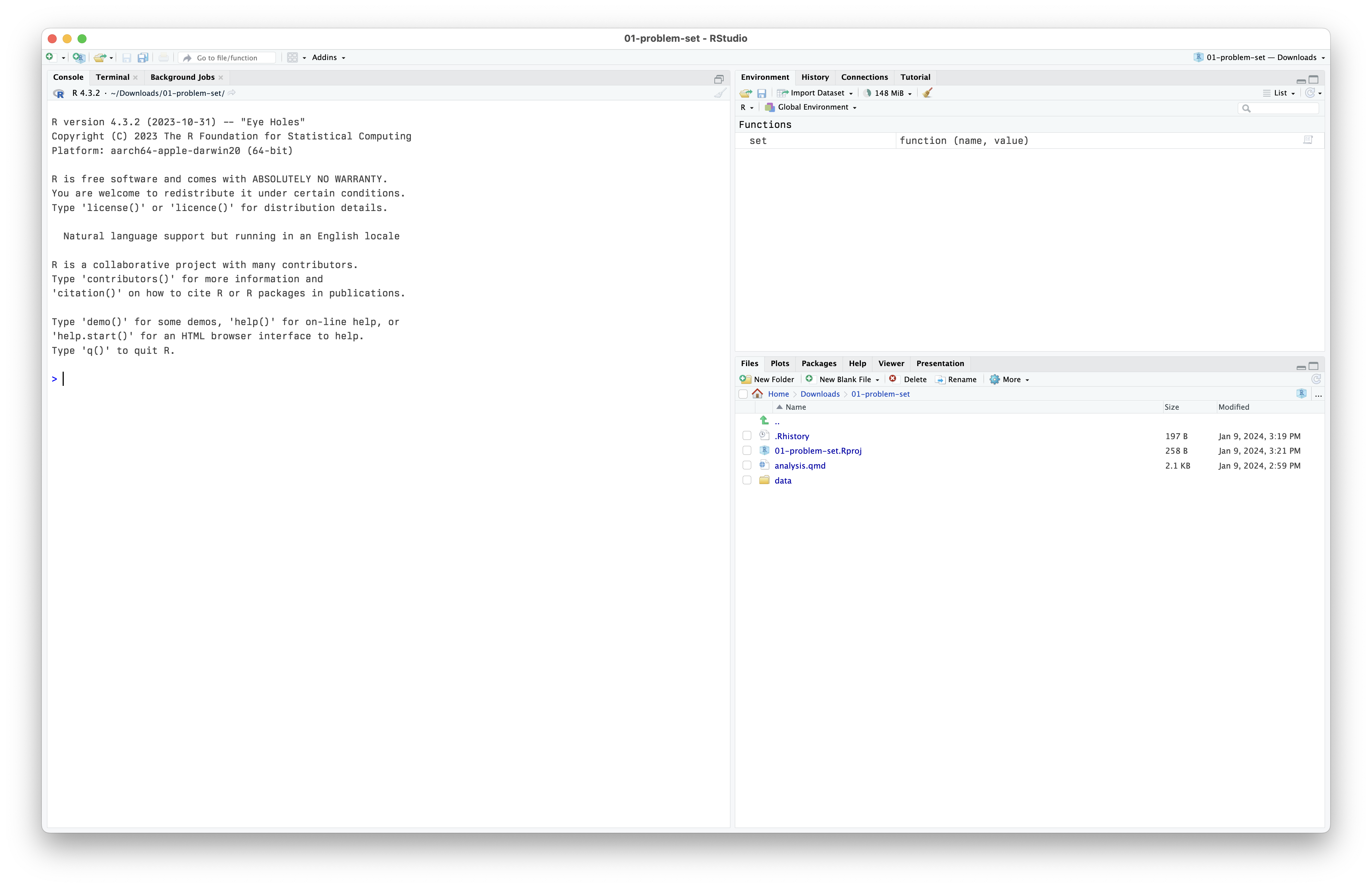
Open it
- Uncompress the Zip file if that doesn’t happen automatically
- Double-click the
01-problem-set.Rprojfile. - RStudio should launch

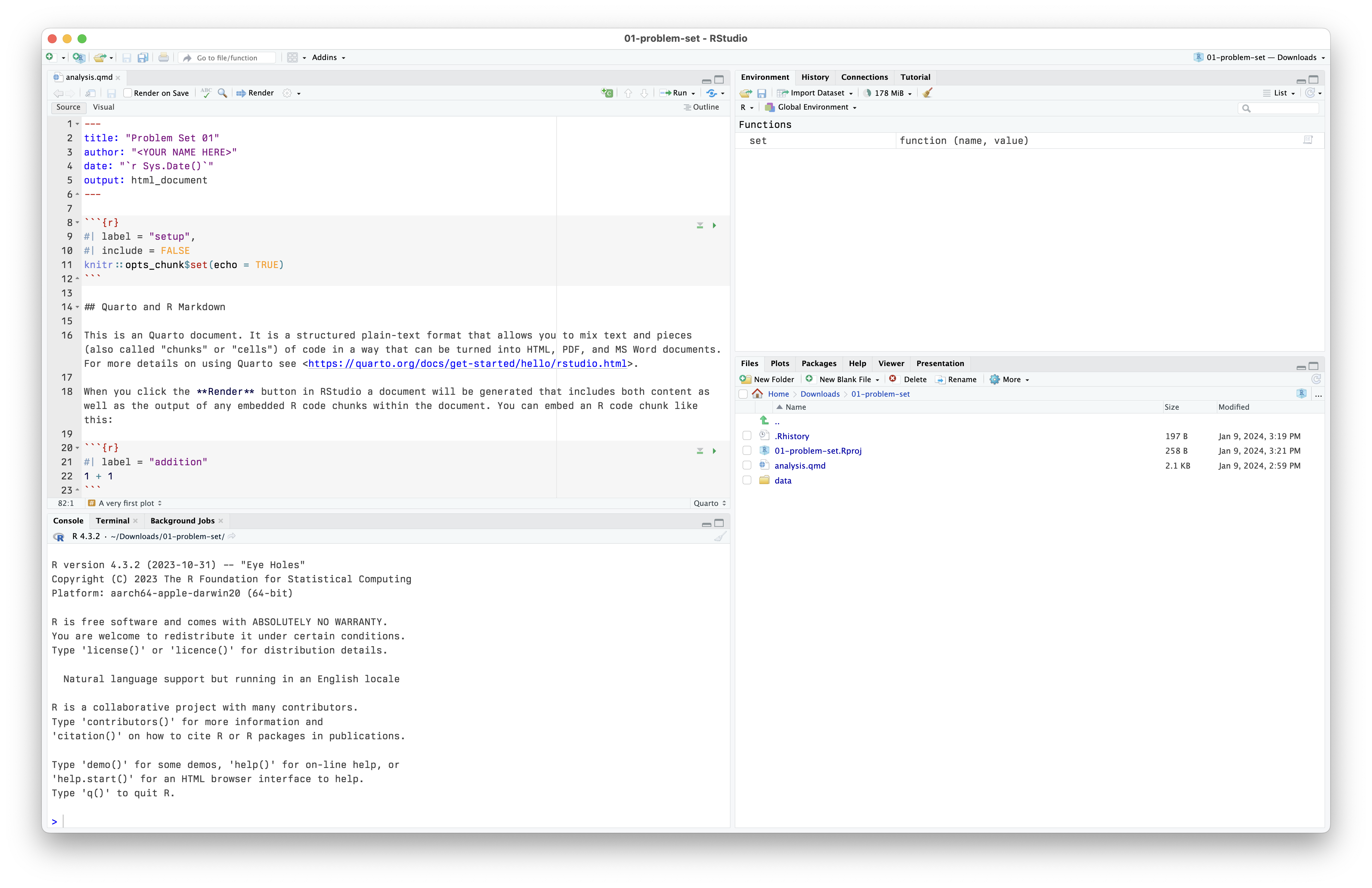
Try rendering the problem set
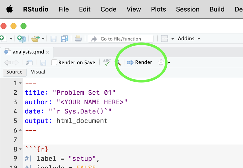
And render your document
Write this out inside the “code chunk” in your notes.
library(tidyverse)
library(gapminder)

p <- ggplot(data = gapminder,
            mapping = aes(x = gdpPercap,
                          y = lifeExp))


p + geom_point()