“Laundry Pile” user model of where things are stored
Where technical computing lives
Windows and pointers.
Multi-tasking, multiple windows.
Exposes and leverages the file system.
Many specialized tools in concert.
Underneath, it’s the 1970s, UNIX, and the command-line.
Cabinets, drawers, and files model of where things are stored
Where technical computing lives
This toolset is by now really good!
Free! Open! Powerful!
Friendly communities! Lots of information! Many resources!
But: grounded in a UI paradigm that is increasingly far away from the everyday use of computing devices
So why do we use this stuff?
“Office” vs “Engineering” approaches
What is “real” in your project?
What is the final output?
How is it produced?
How are changes managed?
Different Answers
Office model
Formatted documents are real.
Intermediate outputs are cut and pasted into documents.
Changes are tracked inside files.
Final output is often in the same format you’ve been working in, e.g. a Word file, or a PDF.
Engineering model
Plain-text files are real.
Intermediate outputs are produced via code, often inside documents.
Changes are tracked outside files, at the level of a project.
Final outputs are assembled programmatically and converted to some desired format.
Different strengths and weaknesses
Office model
Everyone knows Word, Excel, or Google Docs.
“Track changes” is powerful and easy.
Hm, I can’t remember how I made this figure
Where did this table of results come from?
Paper_edits_FINAL_kh-1.docx
Engineering model
Plain text is highly portable.
Push button, recreate analysis.
JFC Why can’t I do this simple thing?
Object of type 'closure' is not subsettable
Each approach generates solutions to its own problems
The File System
The traditional analog
The problem is, you probably have never have actually used one of these!
The file cabinet!
The file cabinet!
Index cards
Index cards
Automating information processing
Automating information processing
Automating information processing
Hollerith machines
Hollerith Machines
Hollerith machines
Hollerith machines
Hollerith Operators
Hollerith Operators
IBM punch cards
IBM punch cards
Big Iron
Storage
Storage
Input/Output
A late-model teletype (TTY) machine
Input/Output
The DEC VT-100 Terminal
Input/Output
Back to the file system
File system hierarchy
Stepping back
Your computer stores files and does stuff, or “runs commands”
Files are stored in a large hierarchy of folders
The Finder or Window Manager or File Manager is a visual metaphor for representing this hierarchy of files and for running commands on them. But you can also do these things via text-based commands delivered from a prompt, console, or “command line”.
Software like RStudio has a lot of these “old school” computing elements
Getting to knowR and RStudio
We want to draw graphsreproducibly
Abstraction in software
Less
Easy things are awkward
Hard things are straightforward
Really hard things are possible
Abstraction in software
Less
Easy things are awkward
Hard things are straightforward
Really hard things are possible
More
Easy things are trivial
Hard things are awkward
Really hard things are impossible
Compare
D3
Grid
ggplot
Stata
Excel
The RStudio IDE
An IDE for R
An IDE for Meals
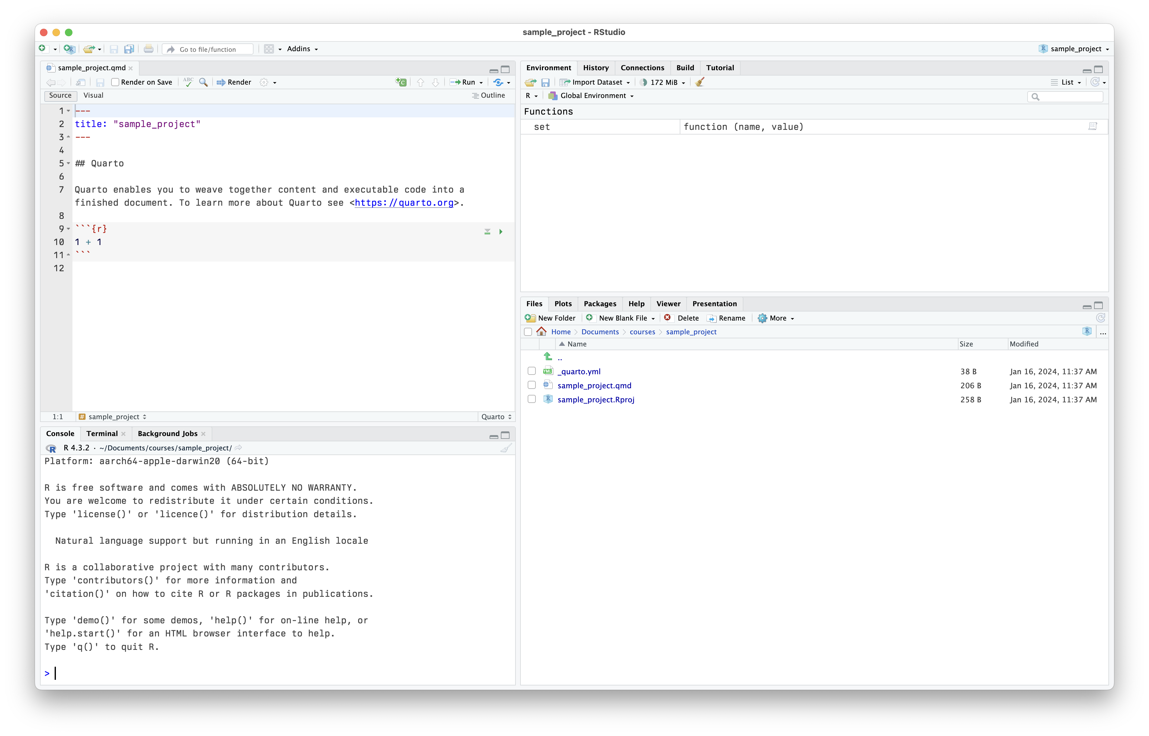
RStudio at startup
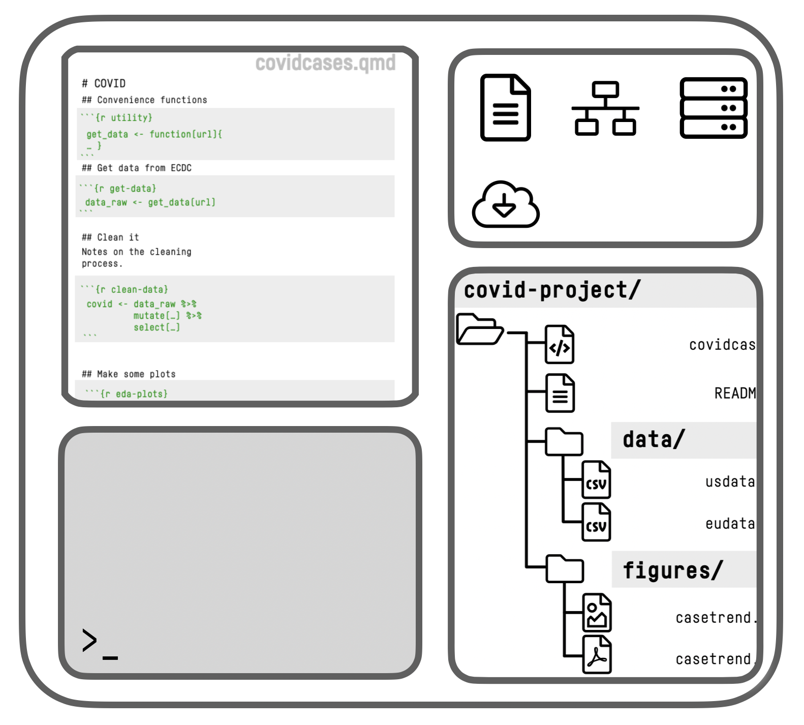
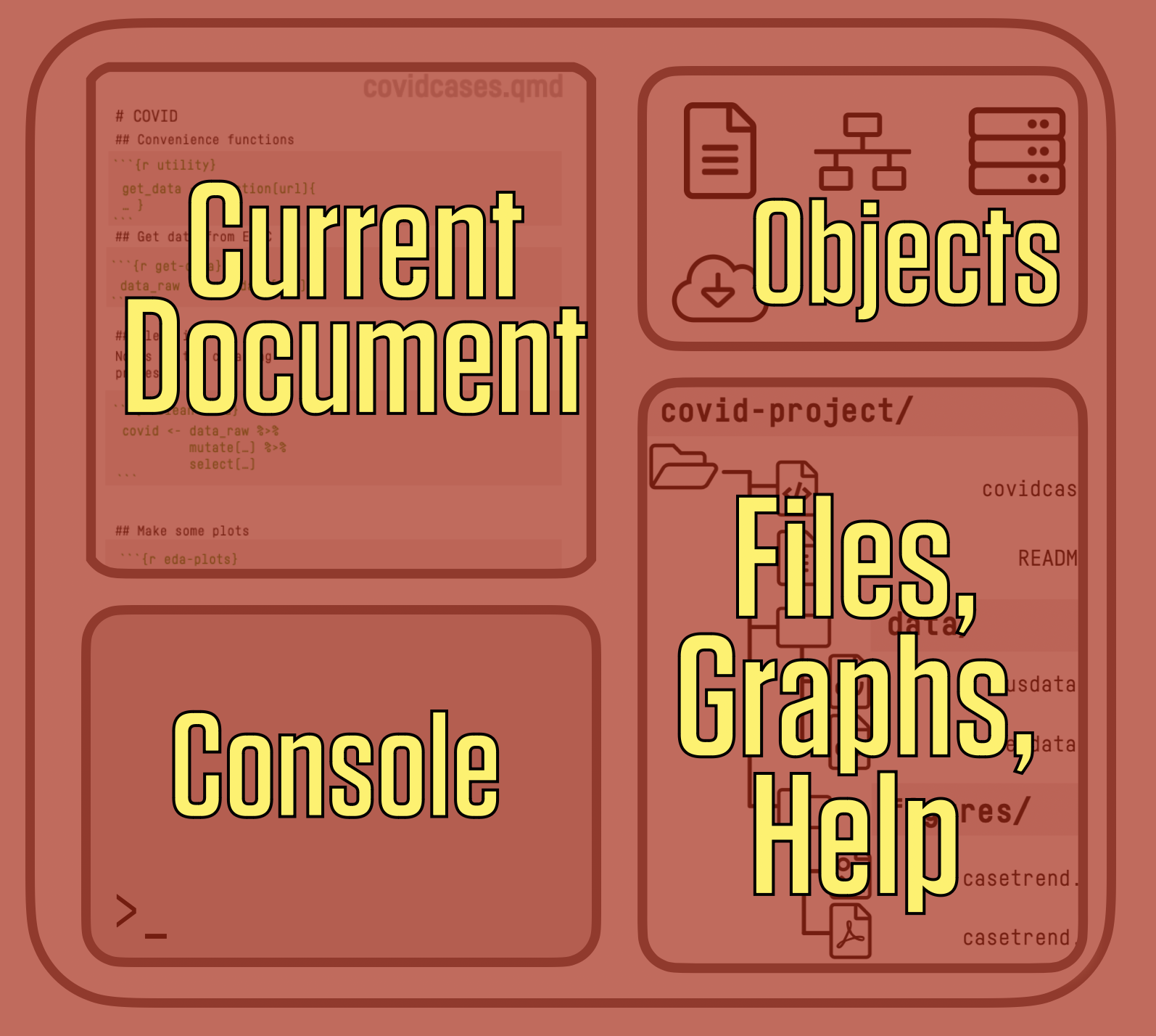
RStudio schematic overview
RStudio schematic overview
Think in terms of Data + Transformations, written out as code, rather than a series of point-and-click steps
Our starting data + our code is what’s “real” in our projects, not the final output or any intermediate objects
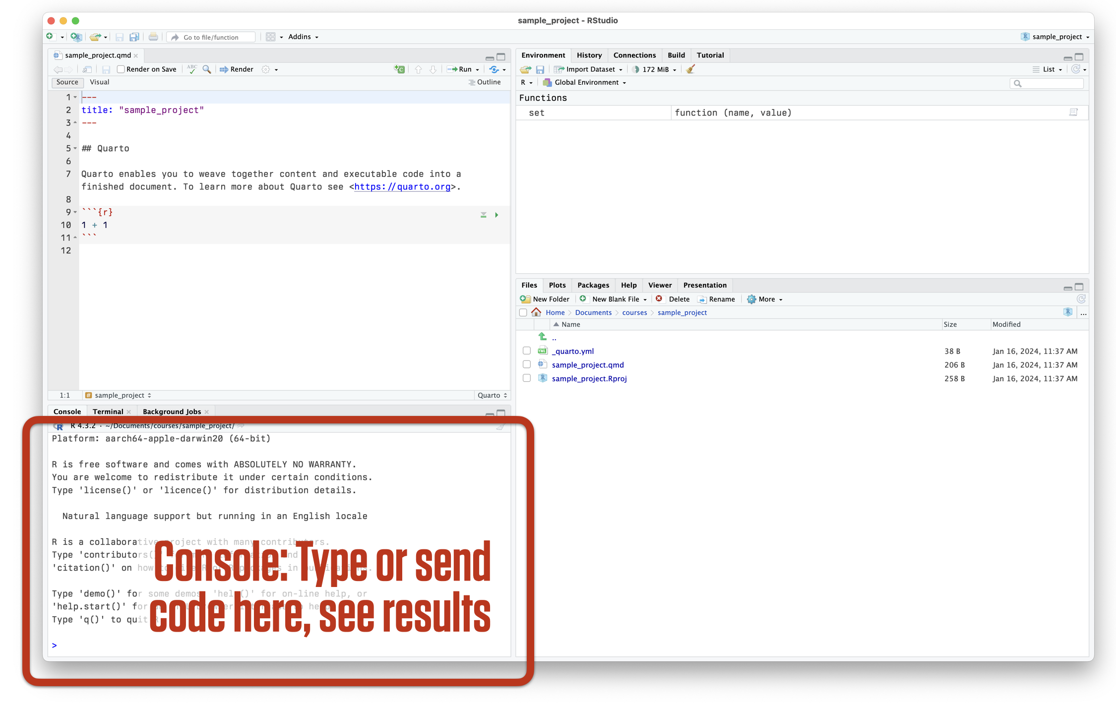
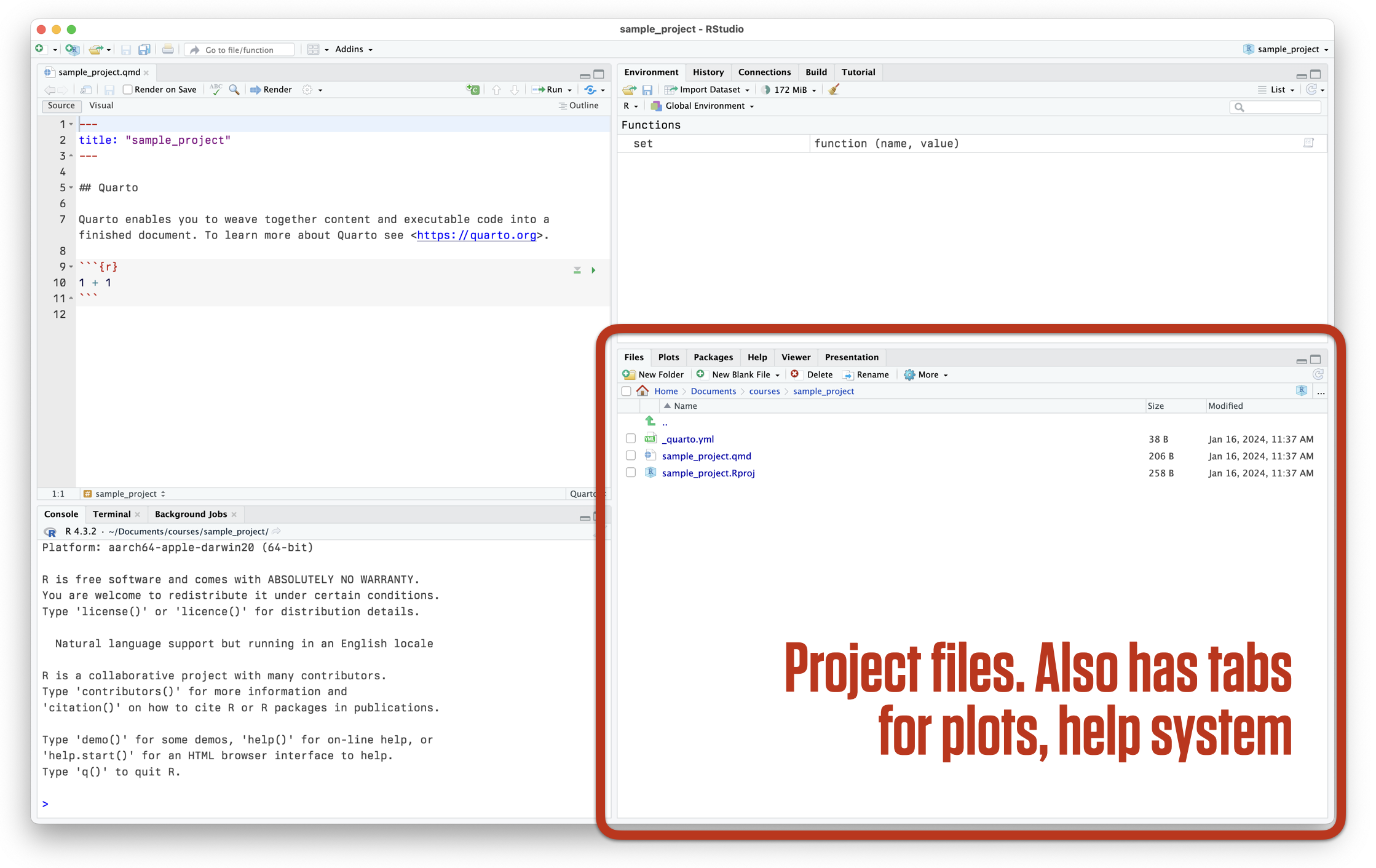
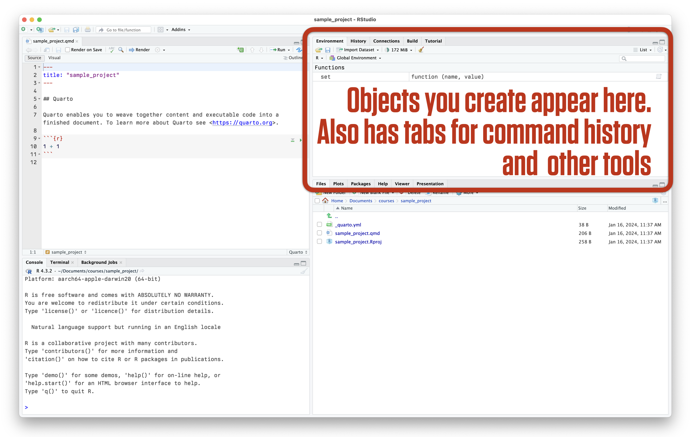
RStudio at startup
RStudio at startup
RStudio at startup
RStudio at startup
RStudio at startup
Use RMarkdown to produce and reproduce work
Where we want to end up
PDF out
Where we want to end up
HTML out
Where we want to end up
Word out
How to get there?
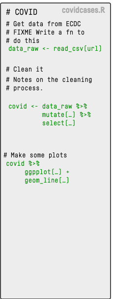
We could write an R script with some notes inside, using it to create some figures and tables, paste them into our document.
This will work, but we can do better.
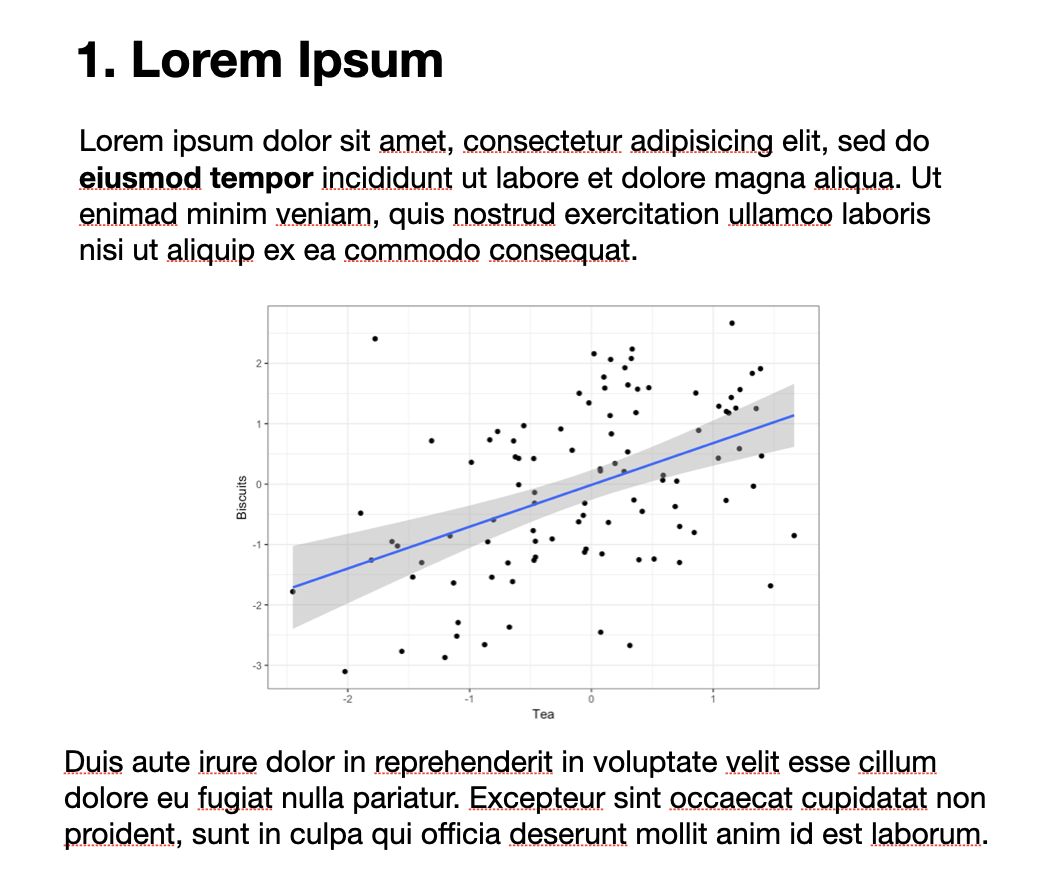
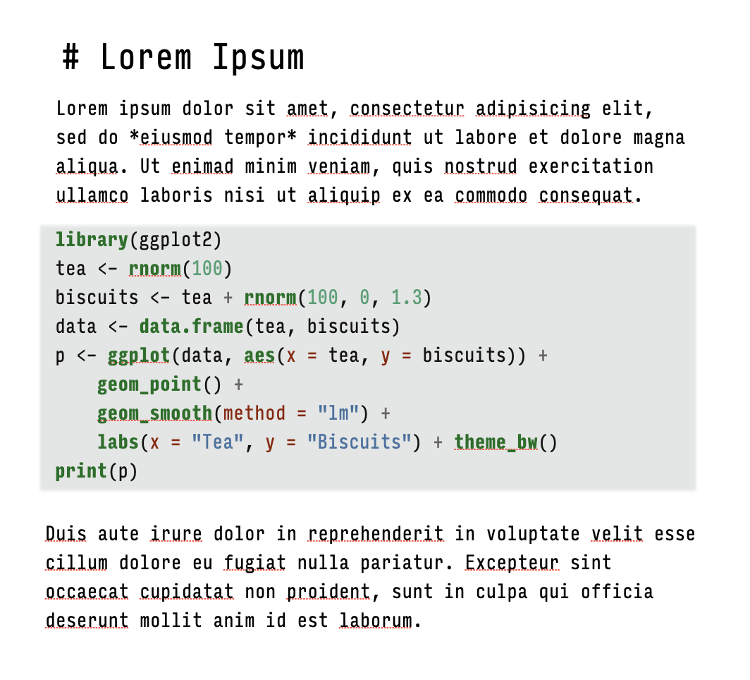
We can make this …
… by writing this
The code gets replaced by its output
Markdown document
Markdown document annotated
This approach has its limitations, but it’s very useful and has many benefits.
This is like learning how to drive a car, or how to cook in a kitchen … or learning to speak a language.
After some orientation to what’s where, you will learn best by doing.
Software is a pain, but you won’t crash the car or burn your house down.
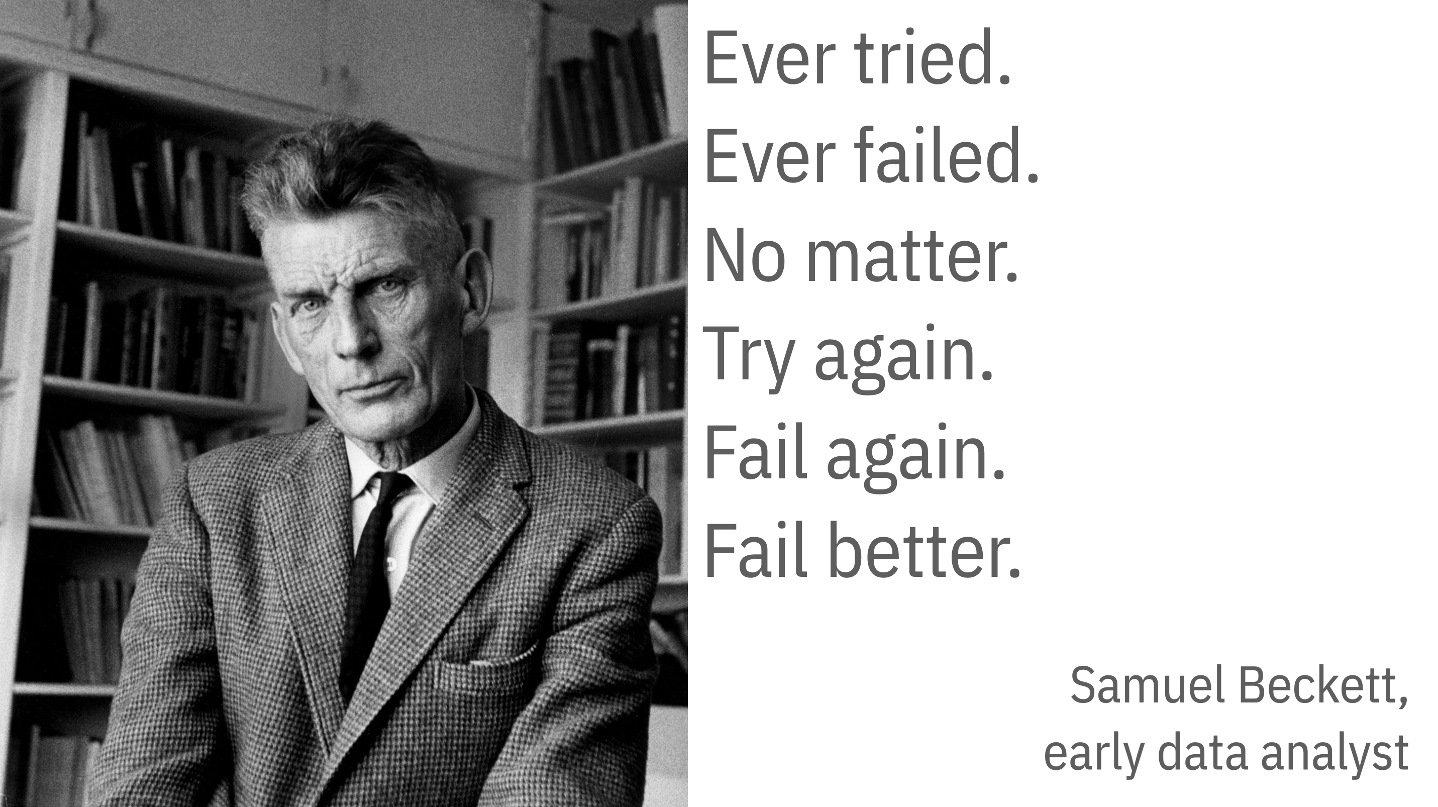
TYPE OUT YOUR CODE BY HAND
Samuel Beckett
GETTING ORIENTED
Loading the tidyverse libraries
library(tidyverse)
The tidyverse has several components.
We’ll return to this message about Conflicts later.
Again, the code and messages you see here is actual R output, produced at the same time as the slide.
Tidyverse components
library(tidyverse)
Loading tidyverse: ggplot2
Loading tidyverse: tibble
Loading tidyverse: tidyr
Loading tidyverse: readr
Loading tidyverse: purrr
Loading tidyverse: dplyr
Call the package and …
<|Draw graphs
<|Nicer data tables
<|Tidy your data
<|Get data into R
<|Fancy Iteration
<|Action verbs for tables
What R looks like
Code you can type and run:
## Inside code chunks, lines beginning with a # character are comments## Comments are ignored by Rmy_numbers <-c(1, 1, 2, 4, 1, 3, 1, 5) # Anything after a # character is ignored as well
Output:
my_numbers
[1] 1 1 2 4 1 3 1 5
This is equivalent to running the code above, typing my_numbers at the console, and hitting enter.
What R looks like
By convention, code output in documents is prefixed by ##
Also by convention, outputting vectors, etc, gets a counter keeping track of the number of elements. For example,
letters
 [1] "a" "b" "c" "d" "e" "f" "g" "h" "i" "j" "k" "l" "m" "n" "o" "p" "q" "r" "s"
[20] "t" "u" "v" "w" "x" "y" "z"
Some things to know about R
0. It’s a calculator
Arithmetic
(31*12) /2^4
[1] 23.25
sqrt(25)
[1] 5
log(100)
[1] 4.60517
log10(100)
[1] 2
0. It’s a calculator
Arithmetic
(31*12) /2^4
[1] 23.25
sqrt(25)
[1] 5
log(100)
[1] 4.60517
log10(100)
[1] 2
Logic
4<10
[1] TRUE
4>2&1>0.5# The "&" means "and"
[1] TRUE
4<2|1>0.5# The "|" means "or"
[1] TRUE
4<2|1<0.5
[1] FALSE
Boolean and Logical operators
Logical equality and inequality (yielding a TRUE or FALSE result) is done with == and !=. Other logical operators include <, >, <=, >=, and ! for negation.
## A logical test2==2# Write `=` twice
[1] TRUE
## This will cause an error, because R will think you are trying to assign a value2=2## Error in 2 = 2 : invalid (do_set) left-hand side to assignment
3!=7# Write `!` and then `=` to make `!=`
[1] TRUE
1. Everything in R has a name
my_numbers # We created this a few minutes ago
[1] 1 1 2 4 1 3 1 5
letters # This one is built-in
 [1] "a" "b" "c" "d" "e" "f" "g" "h" "i" "j" "k" "l" "m" "n" "o" "p" "q" "r" "s"
[20] "t" "u" "v" "w" "x" "y" "z"
pi # Also built-in
[1] 3.141593
Some names are forbidden
Or it’s a really bad idea to try to use them
TRUEFALSEInfNaNNANULLforifwhilebreakfunction
2. Everything is an object
There are a few built-in objects:
letters
 [1] "a" "b" "c" "d" "e" "f" "g" "h" "i" "j" "k" "l" "m" "n" "o" "p" "q" "r" "s"
[20] "t" "u" "v" "w" "x" "y" "z"
pi
[1] 3.141593
LETTERS
 [1] "A" "B" "C" "D" "E" "F" "G" "H" "I" "J" "K" "L" "M" "N" "O" "P" "Q" "R" "S"
[20] "T" "U" "V" "W" "X" "Y" "Z"
3. You can create objects
In fact, this is mostly what we will be doing.
Objects are created by assigning a thing to a name:
## name... gets ... this stuffmy_numbers <-c(1, 2, 3, 1, 3, 5, 25, 10)## name ... gets ... the output of the function `c()`your_numbers <-c(5, 31, 71, 1, 3, 21, 6, 52)
The c() function combines or concatenates things
The assignment operator
The assignment operator performs the action of creating objects
Use a keyboard shortcut to write it:
Press optionand- on a Mac
Press altand- on Windows
Assignment with =
You can use = as well as <- for assignment.
my_numbers =c(1, 2, 3, 1, 3, 5, 25)my_numbers
[1] 1 2 3 1 3 5 25
On the other hand, = has a different meaning when used in functions.
I’m going to use <- for assignment throughout.
Be consistent either way.
4. You do things with functions
## this object... gets ... the output of this functionmy_numbers <-c(1, 2, 3, 1, 3, 5, 25, 10)your_numbers <-c(5, 31, 71, 1, 3, 21, 6, 52)
my_numbers
[1] 1 2 3 1 3 5 25 10
4. You do things with functions
Functions can be identified by the parentheses after their names.
my_numbers
[1] 1 2 3 1 3 5 25 10
## If you run this you'll get an errormean()
What functions usually do
They take inputs to arguments
They perform actions
They produce, or return, outputs
mean(x=my_numbers)
What functions usually do
They take inputs to arguments
They perform actions
They produce, or return, outputs
mean(x=my_numbers)
[1] 6.25
What functions usually do
## Get the mean of what? Of x.## You need to tell the function what x ismean(x = my_numbers)
[1] 6.25
mean(x = your_numbers)
[1] 23.75
What functions usually do
If you don’t name the arguments, R assumes you are providing them in the order the function expects.
mean(your_numbers)
[1] 23.75
What functions usually do
What arguments? Which order? Read the function’s help page
help(mean)
## quicker?mean
How to read an R help page?
What functions usually do
Arguments often tell the function what to do in specific circumstances
We’ll still use nested parentheses quite a bit, often in the context of a function working inside a pipeline. But it’s good not to have too many levels of nesting.
The other pipe: %>%
The Base R pipe operator, |> is a relatively recent addition to R.
Piping operations were originally introduced in a package called called magrittr, where it took the form %>%
The other pipe: %>%
The Base R pipe operator, |> is a relatively recent addition to R.
Piping operations were originally introduced in a package called called magrittr, where it took the form %>%
It’s been so successful, a version of it has been incorporated into Base R. For our puposes, they’re the same.
Functions are bundled into packages
Packages are loaded into your working environment using the library() function:
## A package containing a dataset rather than functionslibrary(gapminder)gapminder
# A tibble: 1,704 × 6
   country     continent  year lifeExp      pop gdpPercap
   <fct>       <fct>     <int>   <dbl>    <int>     <dbl>
 1 Afghanistan Asia       1952    28.8  8425333      779.
 2 Afghanistan Asia       1957    30.3  9240934      821.
 3 Afghanistan Asia       1962    32.0 10267083      853.
 4 Afghanistan Asia       1967    34.0 11537966      836.
 5 Afghanistan Asia       1972    36.1 13079460      740.
 6 Afghanistan Asia       1977    38.4 14880372      786.
 7 Afghanistan Asia       1982    39.9 12881816      978.
 8 Afghanistan Asia       1987    40.8 13867957      852.
 9 Afghanistan Asia       1992    41.7 16317921      649.
10 Afghanistan Asia       1997    41.8 22227415      635.
# ℹ 1,694 more rows
Functions are bundled into packages
You need only install a package once (and occasionally update it):
## Do at least once for each package. Once done, not needed each time.install.packages("palmerpenguins", repos ="http://cran.rstudio.com")## Needed sometimes, especially after an R major version upgrade.update.packages(repos ="http://cran.rstudio.com")
Functions are bundled into packages
But you must load the package in each R session before you can access its contents:
## To load a package, usually at the start of your RMarkdown document or script filelibrary(palmerpenguins)penguins
# A tibble: 344 × 8
   species island    bill_length_mm bill_depth_mm flipper_length_mm body_mass_g
   <fct>   <fct>              <dbl>         <dbl>             <int>       <int>
 1 Adelie  Torgersen           39.1          18.7               181        3750
 2 Adelie  Torgersen           39.5          17.4               186        3800
 3 Adelie  Torgersen           40.3          18                 195        3250
 4 Adelie  Torgersen           NA            NA                  NA          NA
 5 Adelie  Torgersen           36.7          19.3               193        3450
 6 Adelie  Torgersen           39.3          20.6               190        3650
 7 Adelie  Torgersen           38.9          17.8               181        3625
 8 Adelie  Torgersen           39.2          19.6               195        4675
 9 Adelie  Torgersen           34.1          18.1               193        3475
10 Adelie  Torgersen           42            20.2               190        4250
# ℹ 334 more rows
# ℹ 2 more variables: sex <fct>, year <int>
Let’s Go!
Like before
library(tidyverse)library(gapminder)p <-ggplot(data = gapminder, mapping =aes(x = gdpPercap, y = lifeExp)) p +geom_point()
What we did
library(tidyverse)library(gapminder)
Load the packages we need: tidyverse and gapminder
What we did
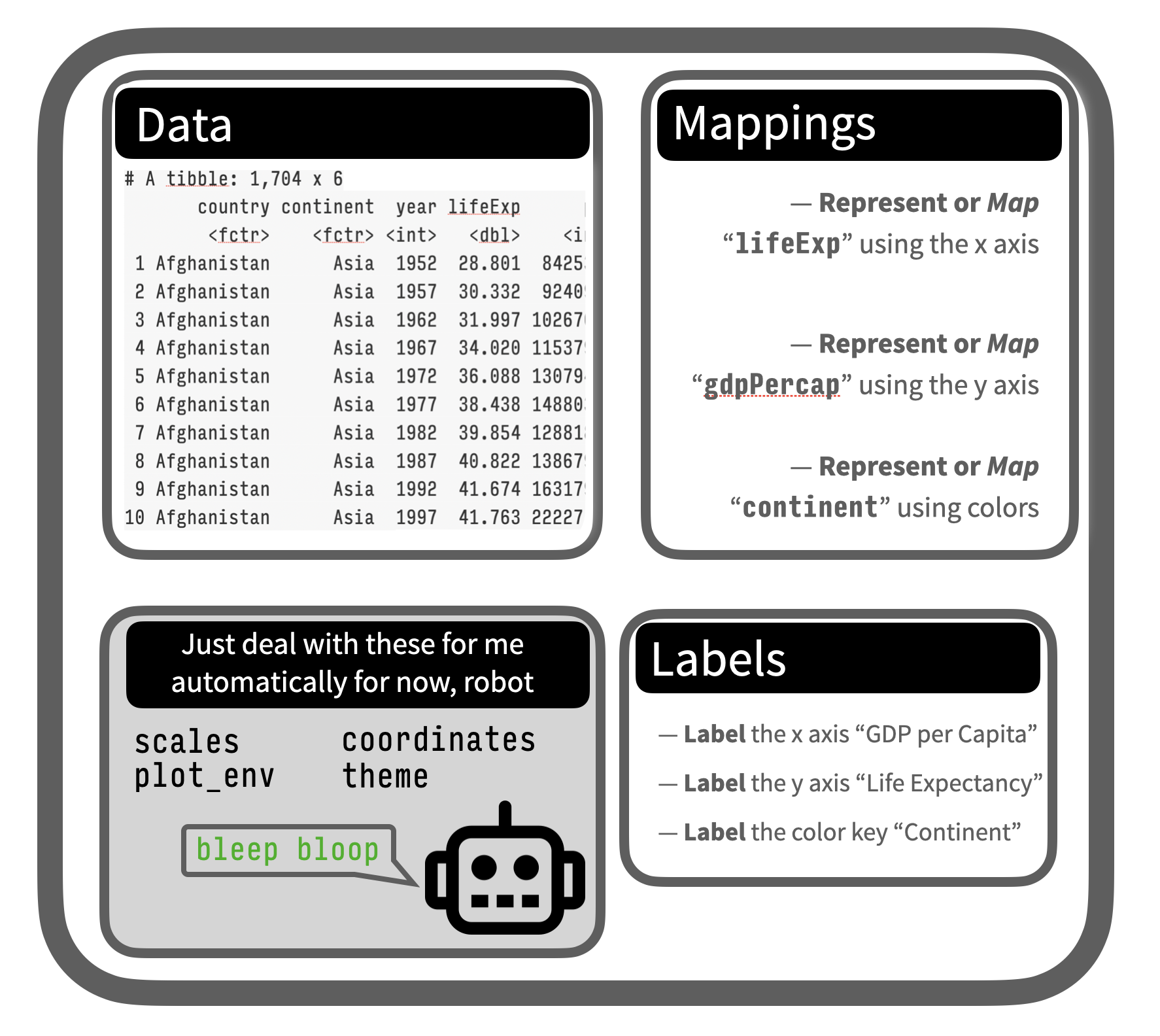
p <-ggplot(data = gapminder, mapping =aes(x = gdpPercap, y = lifeExp))
New object named pgets the output of the ggplot()function, given these arguments
Notice how one of the arguments, mapping, is itself taking the output of a function named aes()
What we did
p +geom_point()
Show me the output of the p object and the geom_point() function.
The + here acts just like the |> pipe, but for ggplot functions only. (This is an accident of history.)
And what is R doing?
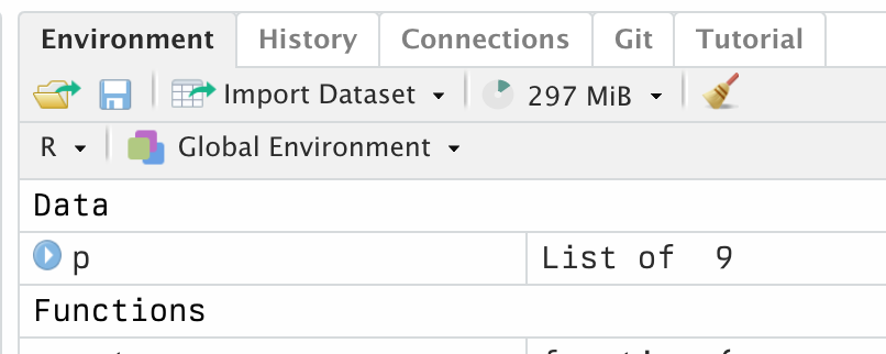
R objects are just lists of stuff to use or things to do
Objects are like Bento Boxes
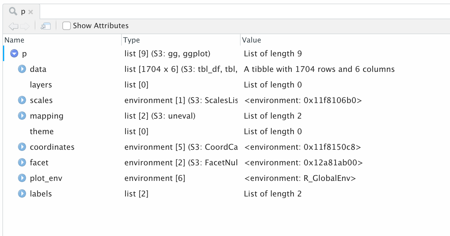
The p object
Peek in with the object inspector
Peek in with the object inspector
Core concepts: mappings + geoms
The core idea, which we’ll focus on more formally next week, is that we have data, arranged in columns, that we want to represent visually on some sort of plot.
That means we need a mapping — a link, a connection, a representation — between things in our table and stuff we can draw. That is what the mapping argument is for.
And we need a geom — a kind of plot, a particular sort of graph — that we draw with that.
Practical examples
Let’s try some live examples …How might we improve or extend this graph based on the data we have? Or how might we look at it differently?