library(here)      # manage file paths
library(socviz)    # data and some useful functions
library(tidyverse) # your friend and mine05 — Show the Right Numbers
Kieran Healy
February 7, 2024
Show the
Right Numbers
with dplyr
Load our libraries
Tidyverse components
library(tidyverse)Loading tidyverse: ggplot2Loading tidyverse: tibbleLoading tidyverse: tidyrLoading tidyverse: readrLoading tidyverse: purrrLoading tidyverse: dplyr
- Load the package and …
<|Draw graphs<|Nicer data tables<|Tidy your data<|Get data into R<|Fancy Iteration<|Action verbs for tables
Other tidyverse components
forcatshavenlubridatereadxlstringrreprex
<|Deal with factors<|Import Stata, SPSS, etc<|Dates, Durations, Times<|Import from spreadsheets<|Strings and Regular Expressions<|Make reproducible examples
Not all of these are attached when we do library(tidyverse)
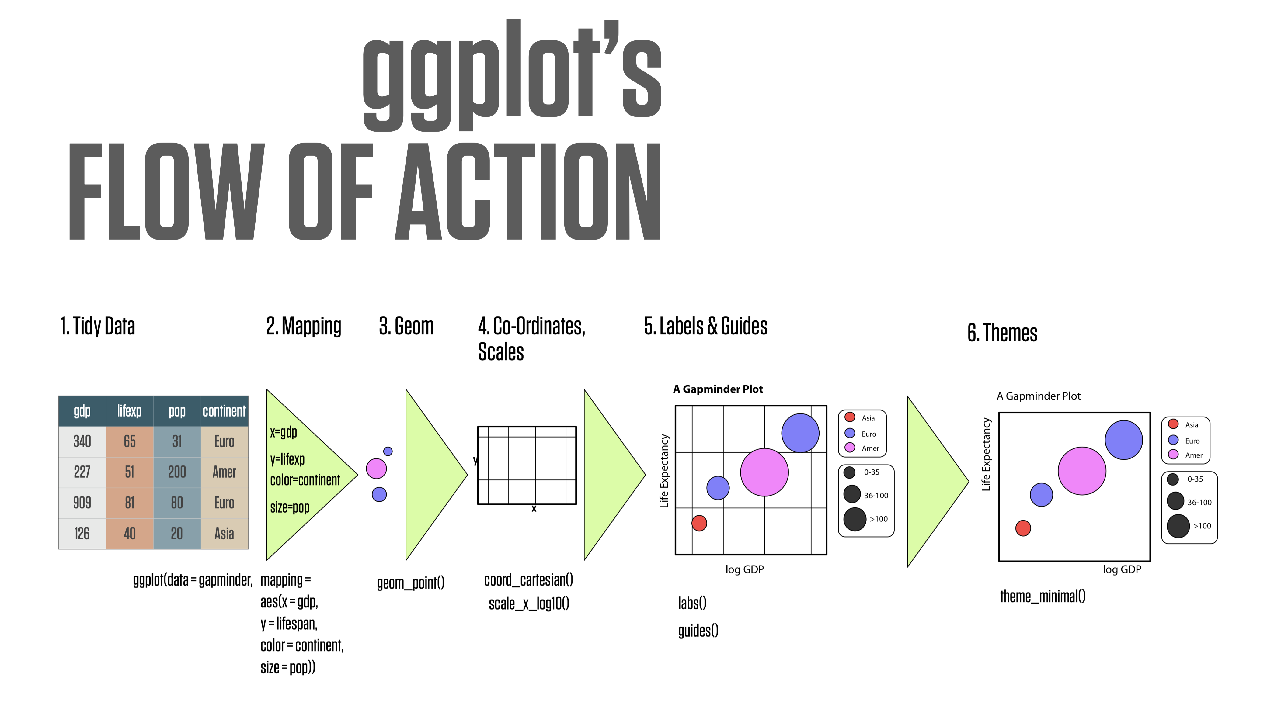
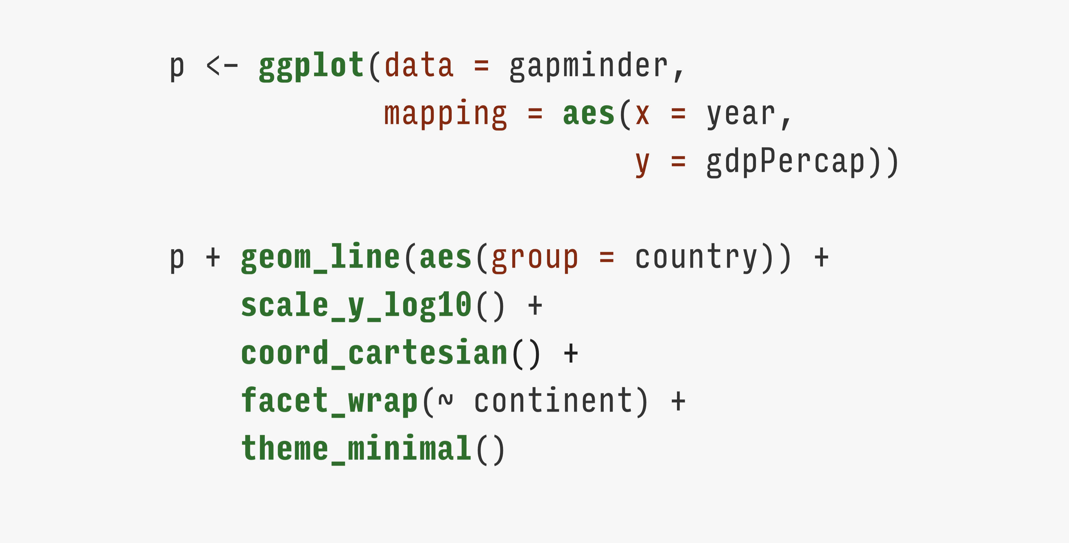
ggplot’s flow of action

Thinking in terms of layers
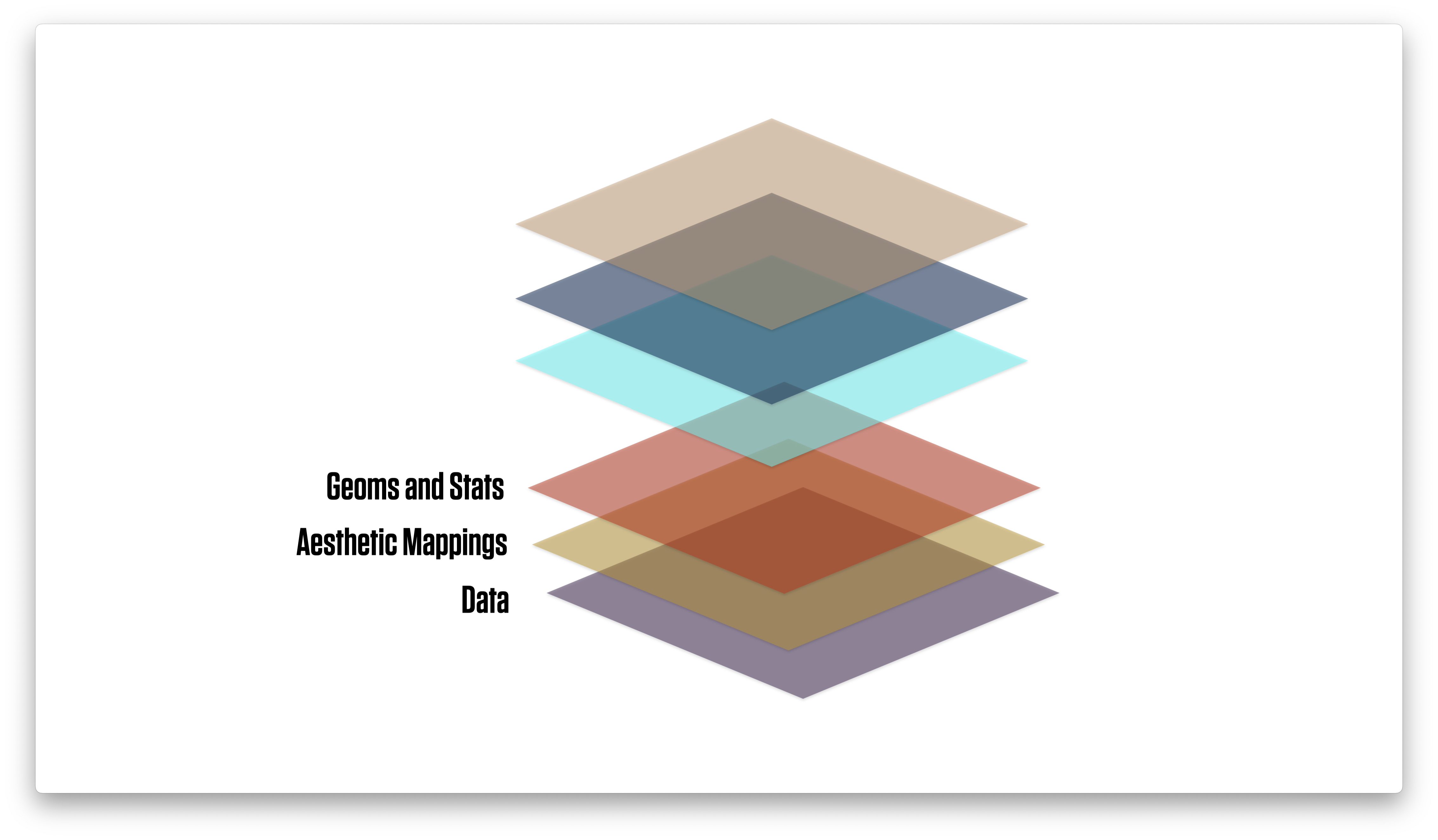
Thinking in terms of layers

Thinking in terms of layers
Feeding data
to ggplot
Transform and summarize first.
Then send your clean tables to ggplot.
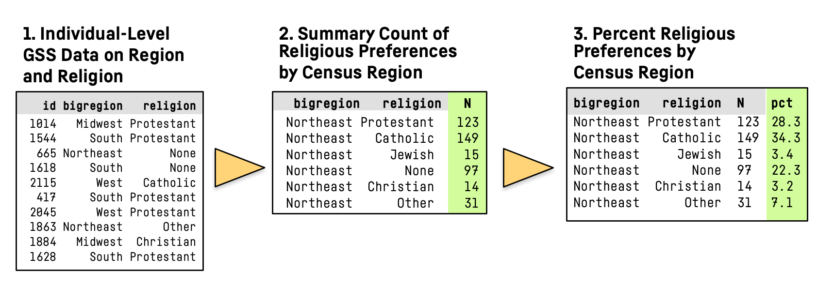
Crosstabulation and beyond
U.S. General Social Survey data
# A tibble: 2,867 × 32
    year    id ballot       age childs sibs   degree race  sex   region income16
   <dbl> <dbl> <labelled> <dbl>  <dbl> <labe> <fct>  <fct> <fct> <fct>  <fct>
 1  2016     1 1             47      3 2      Bache… White Male  New E… $170000…
 2  2016     2 2             61      0 3      High … White Male  New E… $50000 …
 3  2016     3 3             72      2 3      Bache… White Male  New E… $75000 …
 4  2016     4 1             43      4 3      High … White Fema… New E… $170000…
 5  2016     5 3             55      2 2      Gradu… White Fema… New E… $170000…
 6  2016     6 2             53      2 2      Junio… White Fema… New E… $60000 …
 7  2016     7 1             50      2 2      High … White Male  New E… $170000…
 8  2016     8 3             23      3 6      High … Other Fema… Middl… $30000 …
 9  2016     9 1             45      3 5      High … Black Male  Middl… $60000 …
10  2016    10 3             71      4 1      Junio… White Male  Middl… $60000 …
# ℹ 2,857 more rows
# ℹ 21 more variables: relig <fct>, marital <fct>, padeg <fct>, madeg <fct>,
#   partyid <fct>, polviews <fct>, happy <fct>, partners <fct>, grass <fct>,
#   zodiac <fct>, pres12 <labelled>, wtssall <dbl>, income_rc <fct>,
#   agegrp <fct>, ageq <fct>, siblings <fct>, kids <fct>, religion <fct>,
#   bigregion <fct>, partners_rc <fct>, obama <dbl>
We often want summary tables or graphs of data like this.
Two-way tables: Row percents
| bigregion | Protestant | Catholic | Jewish | None | Other | Total |
|---|---|---|---|---|---|---|
| Northeast | 32.4 | 33.3 | 5.5 | 23.0 | 5.7 | 100.0 |
| Midwest | 47.1 | 24.9 | 0.4 | 22.8 | 4.8 | 100.0 |
| South | 62.4 | 15.4 | 1.1 | 16.3 | 4.8 | 100.0 |
| West | 37.7 | 24.6 | 1.6 | 28.5 | 7.6 | 100.0 |
Two-way tables: Column percents
| bigregion | Protestant | Catholic | Jewish | None | Other |
|---|---|---|---|---|---|
| Northeast | 11.5 | 25.0 | 52.9 | 18.1 | 17.6 |
| Midwest | 23.7 | 26.5 | 5.9 | 25.4 | 20.8 |
| South | 47.4 | 24.7 | 21.6 | 27.5 | 31.4 |
| West | 17.4 | 23.9 | 19.6 | 29.1 | 30.2 |
| Total | 100.0 | 100.0 | 100.0 | 100.0 | 100.0 |
Two-way tables: Full marginals
| bigregion | Protestant | Catholic | Jewish | None | Other |
|---|---|---|---|---|---|
| Northeast | 5.5 | 5.7 | 0.9 | 3.9 | 1.0 |
| Midwest | 11.4 | 6.0 | 0.1 | 5.5 | 1.2 |
| South | 22.8 | 5.6 | 0.4 | 6.0 | 1.8 |
| West | 8.4 | 5.4 | 0.4 | 6.3 | 1.7 |
dplyr lets you work with tibbles
Remember, tibbles are tables of data where the columns can be of different types, such as integer, double, logical, character, factor, etc.
We’ll use dplyr to transform and summarize our data.
- We’ll use the pipe operator,
|>, to chain together sequences of actions on our tables.
dplyr’s core verbs
dplyr draws on the logic and language of database queries
Some actions to take on a single table
Group the data at the level we want, such as “Religion by Region” or “Children by School”.
Subset either the rows or columns of or table—i.e. remove them before doing anything.
Mutate the data. That is, change something at the current level of grouping. Mutating adds new columns to the table, or changes the content of an existing column. It never changes the number of rows.
Summarize or aggregate the data. That is, make something new at a higher level of grouping. E.g., calculate means or counts by some grouping variable. This will generally result in a smaller, summary table. Usually this will have the same number of rows as there are groups being summarized.
For each action there’s a function
Group using group_by().
Subset has one action for rows and one for columns. We filter() rows and select() columns.
Mutate tables (i.e. add new columns, or re-make existing ones) using mutate().
Summarize tables (i.e. perform aggregating calculations) using summarize().
Group and Summarize
General Social Survey data: gss_sm
# A tibble: 2,867 × 32
    year    id ballot       age childs sibs   degree race  sex   region income16
   <dbl> <dbl> <labelled> <dbl>  <dbl> <labe> <fct>  <fct> <fct> <fct>  <fct>
 1  2016     1 1             47      3 2      Bache… White Male  New E… $170000…
 2  2016     2 2             61      0 3      High … White Male  New E… $50000 …
 3  2016     3 3             72      2 3      Bache… White Male  New E… $75000 …
 4  2016     4 1             43      4 3      High … White Fema… New E… $170000…
 5  2016     5 3             55      2 2      Gradu… White Fema… New E… $170000…
 6  2016     6 2             53      2 2      Junio… White Fema… New E… $60000 …
 7  2016     7 1             50      2 2      High … White Male  New E… $170000…
 8  2016     8 3             23      3 6      High … Other Fema… Middl… $30000 …
 9  2016     9 1             45      3 5      High … Black Male  Middl… $60000 …
10  2016    10 3             71      4 1      Junio… White Male  Middl… $60000 …
# ℹ 2,857 more rows
# ℹ 21 more variables: relig <fct>, marital <fct>, padeg <fct>, madeg <fct>,
#   partyid <fct>, polviews <fct>, happy <fct>, partners <fct>, grass <fct>,
#   zodiac <fct>, pres12 <labelled>, wtssall <dbl>, income_rc <fct>,
#   agegrp <fct>, ageq <fct>, siblings <fct>, kids <fct>, religion <fct>,
#   bigregion <fct>, partners_rc <fct>, obama <dbl>
Notice how the tibble already tells us a lot.
Summarizing a Table
- Here’s what we’re going to do:
Summarizing a Table
# A tibble: 2,867 × 3
      id bigregion religion
   <dbl> <fct>     <fct>
 1     1 Northeast None
 2     2 Northeast None
 3     3 Northeast Catholic
 4     4 Northeast Catholic
 5     5 Northeast None
 6     6 Northeast None
 7     7 Northeast None
 8     8 Northeast Catholic
 9     9 Northeast Protestant
10    10 Northeast None
# ℹ 2,857 more rows
We’re just taking a look at the relevant columns here.
Group by one column or variable
# A tibble: 2,867 × 32
# Groups:   bigregion [4]
    year    id ballot       age childs sibs   degree race  sex   region income16
   <dbl> <dbl> <labelled> <dbl>  <dbl> <labe> <fct>  <fct> <fct> <fct>  <fct>
 1  2016     1 1             47      3 2      Bache… White Male  New E… $170000…
 2  2016     2 2             61      0 3      High … White Male  New E… $50000 …
 3  2016     3 3             72      2 3      Bache… White Male  New E… $75000 …
 4  2016     4 1             43      4 3      High … White Fema… New E… $170000…
 5  2016     5 3             55      2 2      Gradu… White Fema… New E… $170000…
 6  2016     6 2             53      2 2      Junio… White Fema… New E… $60000 …
 7  2016     7 1             50      2 2      High … White Male  New E… $170000…
 8  2016     8 3             23      3 6      High … Other Fema… Middl… $30000 …
 9  2016     9 1             45      3 5      High … Black Male  Middl… $60000 …
10  2016    10 3             71      4 1      Junio… White Male  Middl… $60000 …
# ℹ 2,857 more rows
# ℹ 21 more variables: relig <fct>, marital <fct>, padeg <fct>, madeg <fct>,
#   partyid <fct>, polviews <fct>, happy <fct>, partners <fct>, grass <fct>,
#   zodiac <fct>, pres12 <labelled>, wtssall <dbl>, income_rc <fct>,
#   agegrp <fct>, ageq <fct>, siblings <fct>, kids <fct>, religion <fct>,
#   bigregion <fct>, partners_rc <fct>, obama <dbl>
Grouping just changes the logical structure of the tibble.
Group and summarize by one column
# A tibble: 2,867 × 32
    year    id ballot       age childs sibs   degree race  sex   region income16
   <dbl> <dbl> <labelled> <dbl>  <dbl> <labe> <fct>  <fct> <fct> <fct>  <fct>
 1  2016     1 1             47      3 2      Bache… White Male  New E… $170000…
 2  2016     2 2             61      0 3      High … White Male  New E… $50000 …
 3  2016     3 3             72      2 3      Bache… White Male  New E… $75000 …
 4  2016     4 1             43      4 3      High … White Fema… New E… $170000…
 5  2016     5 3             55      2 2      Gradu… White Fema… New E… $170000…
 6  2016     6 2             53      2 2      Junio… White Fema… New E… $60000 …
 7  2016     7 1             50      2 2      High … White Male  New E… $170000…
 8  2016     8 3             23      3 6      High … Other Fema… Middl… $30000 …
 9  2016     9 1             45      3 5      High … Black Male  Middl… $60000 …
10  2016    10 3             71      4 1      Junio… White Male  Middl… $60000 …
# ℹ 2,857 more rows
# ℹ 21 more variables: relig <fct>, marital <fct>, padeg <fct>, madeg <fct>,
#   partyid <fct>, polviews <fct>, happy <fct>, partners <fct>, grass <fct>,
#   zodiac <fct>, pres12 <labelled>, wtssall <dbl>, income_rc <fct>,
#   agegrp <fct>, ageq <fct>, siblings <fct>, kids <fct>, religion <fct>,
#   bigregion <fct>, partners_rc <fct>, obama <dbl>
Group and summarize by one column
# A tibble: 2,867 × 32
# Groups:   bigregion [4]
    year    id ballot       age childs sibs   degree race  sex   region income16
   <dbl> <dbl> <labelled> <dbl>  <dbl> <labe> <fct>  <fct> <fct> <fct>  <fct>
 1  2016     1 1             47      3 2      Bache… White Male  New E… $170000…
 2  2016     2 2             61      0 3      High … White Male  New E… $50000 …
 3  2016     3 3             72      2 3      Bache… White Male  New E… $75000 …
 4  2016     4 1             43      4 3      High … White Fema… New E… $170000…
 5  2016     5 3             55      2 2      Gradu… White Fema… New E… $170000…
 6  2016     6 2             53      2 2      Junio… White Fema… New E… $60000 …
 7  2016     7 1             50      2 2      High … White Male  New E… $170000…
 8  2016     8 3             23      3 6      High … Other Fema… Middl… $30000 …
 9  2016     9 1             45      3 5      High … Black Male  Middl… $60000 …
10  2016    10 3             71      4 1      Junio… White Male  Middl… $60000 …
# ℹ 2,857 more rows
# ℹ 21 more variables: relig <fct>, marital <fct>, padeg <fct>, madeg <fct>,
#   partyid <fct>, polviews <fct>, happy <fct>, partners <fct>, grass <fct>,
#   zodiac <fct>, pres12 <labelled>, wtssall <dbl>, income_rc <fct>,
#   agegrp <fct>, ageq <fct>, siblings <fct>, kids <fct>, religion <fct>,
#   bigregion <fct>, partners_rc <fct>, obama <dbl>
Group and summarize by one column
# A tibble: 4 × 2
  bigregion total
  <fct>     <int>
1 Northeast   488
2 Midwest     695
3 South      1052
4 West        632
The function n() counts up the rows within each group.
You get as many rows back as there were groups.
All the other columns are dropped in the summary operation
Your original gss_sm table is untouched
Group and summarize by two columns
# A tibble: 2,867 × 32
    year    id ballot       age childs sibs   degree race  sex   region income16
   <dbl> <dbl> <labelled> <dbl>  <dbl> <labe> <fct>  <fct> <fct> <fct>  <fct>
 1  2016     1 1             47      3 2      Bache… White Male  New E… $170000…
 2  2016     2 2             61      0 3      High … White Male  New E… $50000 …
 3  2016     3 3             72      2 3      Bache… White Male  New E… $75000 …
 4  2016     4 1             43      4 3      High … White Fema… New E… $170000…
 5  2016     5 3             55      2 2      Gradu… White Fema… New E… $170000…
 6  2016     6 2             53      2 2      Junio… White Fema… New E… $60000 …
 7  2016     7 1             50      2 2      High … White Male  New E… $170000…
 8  2016     8 3             23      3 6      High … Other Fema… Middl… $30000 …
 9  2016     9 1             45      3 5      High … Black Male  Middl… $60000 …
10  2016    10 3             71      4 1      Junio… White Male  Middl… $60000 …
# ℹ 2,857 more rows
# ℹ 21 more variables: relig <fct>, marital <fct>, padeg <fct>, madeg <fct>,
#   partyid <fct>, polviews <fct>, happy <fct>, partners <fct>, grass <fct>,
#   zodiac <fct>, pres12 <labelled>, wtssall <dbl>, income_rc <fct>,
#   agegrp <fct>, ageq <fct>, siblings <fct>, kids <fct>, religion <fct>,
#   bigregion <fct>, partners_rc <fct>, obama <dbl>
Group and summarize by two columns
# A tibble: 2,867 × 32
# Groups: bigregion, religion [24]
year id ballot age childs sibs degree race sex region income16
<dbl> <dbl> <labelled> <dbl> <dbl> <labe> <fct> <fct> <fct> <fct> <fct>
1 2016 1 1 47 3 2 Bache… White Male New E… $170000…
2 2016 2 2 61 0 3 High … White Male New E… $50000 …
3 2016 3 3 72 2 3 Bache… White Male New E… $75000 …
4 2016 4 1 43 4 3 High … White Fema… New E… $170000…
5 2016 5 3 55 2 2 Gradu… White Fema… New E… $170000…
6 2016 6 2 53 2 2 Junio… White Fema… New E… $60000 …
7 2016 7 1 50 2 2 High … White Male New E… $170000…
8 2016 8 3 23 3 6 High … Other Fema… Middl… $30000 …
9 2016 9 1 45 3 5 High … Black Male Middl… $60000 …
10 2016 10 3 71 4 1 Junio… White Male Middl… $60000 …
# ℹ 2,857 more rows
# ℹ 21 more variables: relig <fct>, marital <fct>, padeg <fct>, madeg <fct>,
# partyid <fct>, polviews <fct>, happy <fct>, partners <fct>, grass <fct>,
# zodiac <fct>, pres12 <labelled>, wtssall <dbl>, income_rc <fct>,
# agegrp <fct>, ageq <fct>, siblings <fct>, kids <fct>, religion <fct>,
# bigregion <fct>, partners_rc <fct>, obama <dbl>Group and summarize by two columns
# A tibble: 24 × 3
# Groups: bigregion [4]
bigregion religion total
<fct> <fct> <int>
1 Northeast Protestant 158
2 Northeast Catholic 162
3 Northeast Jewish 27
4 Northeast None 112
5 Northeast Other 28
6 Northeast <NA> 1
7 Midwest Protestant 325
8 Midwest Catholic 172
9 Midwest Jewish 3
10 Midwest None 157
# ℹ 14 more rowsThe function n() counts up the rows within the groups.
Again, there are as many rows as there were groups. So the “innermost” (i.e. the rightmost) group “disappears” or is “rolled up”.
In this case the tibble out the other side is still grouped at the next level of grouping, here bigregion.
Calculate frequencies
# A tibble: 2,867 × 32
year id ballot age childs sibs degree race sex region income16
<dbl> <dbl> <labelled> <dbl> <dbl> <labe> <fct> <fct> <fct> <fct> <fct>
1 2016 1 1 47 3 2 Bache… White Male New E… $170000…
2 2016 2 2 61 0 3 High … White Male New E… $50000 …
3 2016 3 3 72 2 3 Bache… White Male New E… $75000 …
4 2016 4 1 43 4 3 High … White Fema… New E… $170000…
5 2016 5 3 55 2 2 Gradu… White Fema… New E… $170000…
6 2016 6 2 53 2 2 Junio… White Fema… New E… $60000 …
7 2016 7 1 50 2 2 High … White Male New E… $170000…
8 2016 8 3 23 3 6 High … Other Fema… Middl… $30000 …
9 2016 9 1 45 3 5 High … Black Male Middl… $60000 …
10 2016 10 3 71 4 1 Junio… White Male Middl… $60000 …
# ℹ 2,857 more rows
# ℹ 21 more variables: relig <fct>, marital <fct>, padeg <fct>, madeg <fct>,
# partyid <fct>, polviews <fct>, happy <fct>, partners <fct>, grass <fct>,
# zodiac <fct>, pres12 <labelled>, wtssall <dbl>, income_rc <fct>,
# agegrp <fct>, ageq <fct>, siblings <fct>, kids <fct>, religion <fct>,
# bigregion <fct>, partners_rc <fct>, obama <dbl>Calculate frequencies
# A tibble: 2,867 × 32
# Groups: bigregion, religion [24]
year id ballot age childs sibs degree race sex region income16
<dbl> <dbl> <labelled> <dbl> <dbl> <labe> <fct> <fct> <fct> <fct> <fct>
1 2016 1 1 47 3 2 Bache… White Male New E… $170000…
2 2016 2 2 61 0 3 High … White Male New E… $50000 …
3 2016 3 3 72 2 3 Bache… White Male New E… $75000 …
4 2016 4 1 43 4 3 High … White Fema… New E… $170000…
5 2016 5 3 55 2 2 Gradu… White Fema… New E… $170000…
6 2016 6 2 53 2 2 Junio… White Fema… New E… $60000 …
7 2016 7 1 50 2 2 High … White Male New E… $170000…
8 2016 8 3 23 3 6 High … Other Fema… Middl… $30000 …
9 2016 9 1 45 3 5 High … Black Male Middl… $60000 …
10 2016 10 3 71 4 1 Junio… White Male Middl… $60000 …
# ℹ 2,857 more rows
# ℹ 21 more variables: relig <fct>, marital <fct>, padeg <fct>, madeg <fct>,
# partyid <fct>, polviews <fct>, happy <fct>, partners <fct>, grass <fct>,
# zodiac <fct>, pres12 <labelled>, wtssall <dbl>, income_rc <fct>,
# agegrp <fct>, ageq <fct>, siblings <fct>, kids <fct>, religion <fct>,
# bigregion <fct>, partners_rc <fct>, obama <dbl>Calculate frequencies
# A tibble: 24 × 3
# Groups: bigregion [4]
bigregion religion total
<fct> <fct> <int>
1 Northeast Protestant 158
2 Northeast Catholic 162
3 Northeast Jewish 27
4 Northeast None 112
5 Northeast Other 28
6 Northeast <NA> 1
7 Midwest Protestant 325
8 Midwest Catholic 172
9 Midwest Jewish 3
10 Midwest None 157
# ℹ 14 more rowsCalculate frequencies
# A tibble: 24 × 5
# Groups: bigregion [4]
bigregion religion total freq pct
<fct> <fct> <int> <dbl> <dbl>
1 Northeast Protestant 158 0.324 32.4
2 Northeast Catholic 162 0.332 33.2
3 Northeast Jewish 27 0.0553 5.5
4 Northeast None 112 0.230 23
5 Northeast Other 28 0.0574 5.7
6 Northeast <NA> 1 0.00205 0.2
7 Midwest Protestant 325 0.468 46.8
8 Midwest Catholic 172 0.247 24.7
9 Midwest Jewish 3 0.00432 0.4
10 Midwest None 157 0.226 22.6
# ℹ 14 more rowsThe function n() counts up the rows
Which rows? The ones fed down the pipeline
Summing over the innermost (i.e. the rightmost) group.
Pipelines carry assumptions forward
gss_sm |>
group_by(bigregion, religion) |>
summarize(total = n()) |>
mutate(freq = total / sum(total),
pct = round((freq*100), 1))# A tibble: 24 × 5
# Groups: bigregion [4]
bigregion religion total freq pct
<fct> <fct> <int> <dbl> <dbl>
1 Northeast Protestant 158 0.324 32.4
2 Northeast Catholic 162 0.332 33.2
3 Northeast Jewish 27 0.0553 5.5
4 Northeast None 112 0.230 23
5 Northeast Other 28 0.0574 5.7
6 Northeast <NA> 1 0.00205 0.2
7 Midwest Protestant 325 0.468 46.8
8 Midwest Catholic 172 0.247 24.7
9 Midwest Jewish 3 0.00432 0.4
10 Midwest None 157 0.226 22.6
# ℹ 14 more rowsGroups are carried forward till summarized or explicitly ungrouped
Summary calculations are done on the innermost group, which then “disappears”.
Pipelines carry assumptions forward
gss_sm |>
  group_by(bigregion, religion) |>
summarize(total = n()) |>
mutate(freq = total / sum(total),
pct = round((freq*100), 1)) # A tibble: 24 × 5
# Groups: bigregion [4]
bigregion religion total freq pct
<fct> <fct> <int> <dbl> <dbl>
1 Northeast Protestant 158 0.324 32.4
2 Northeast Catholic 162 0.332 33.2
3 Northeast Jewish 27 0.0553 5.5
4 Northeast None 112 0.230 23
5 Northeast Other 28 0.0574 5.7
6 Northeast <NA> 1 0.00205 0.2
7 Midwest Protestant 325 0.468 46.8
8 Midwest Catholic 172 0.247 24.7
9 Midwest Jewish 3 0.00432 0.4
10 Midwest None 157 0.226 22.6
# ℹ 14 more rowsmutate() is quite clever. See how we can immediately use freq, even though we are creating it in the same mutate() expression.
Convenience functions
gss_sm |>
group_by(bigregion, religion) |>
summarize(total = n()) |>
mutate(freq = total / sum(total),
pct = round((freq*100), 1)) # A tibble: 24 × 5
# Groups: bigregion [4]
bigregion religion total freq pct
<fct> <fct> <int> <dbl> <dbl>
1 Northeast Protestant 158 0.324 32.4
2 Northeast Catholic 162 0.332 33.2
3 Northeast Jewish 27 0.0553 5.5
4 Northeast None 112 0.230 23
5 Northeast Other 28 0.0574 5.7
6 Northeast <NA> 1 0.00205 0.2
7 Midwest Protestant 325 0.468 46.8
8 Midwest Catholic 172 0.247 24.7
9 Midwest Jewish 3 0.00432 0.4
10 Midwest None 157 0.226 22.6
# ℹ 14 more rowsWe’re going to be doing this group_by() … n() step a lot. Some shorthand for it would be useful.
Three options for counting up rows
- Use
n()
# A tibble: 24 × 3
# Groups: bigregion [4]
bigregion religion n
<fct> <fct> <int>
1 Northeast Protestant 158
2 Northeast Catholic 162
3 Northeast Jewish 27
4 Northeast None 112
5 Northeast Other 28
6 Northeast <NA> 1
7 Midwest Protestant 325
8 Midwest Catholic 172
9 Midwest Jewish 3
10 Midwest None 157
# ℹ 14 more rows- Group it yourself; result is grouped.
- Use
tally()
# A tibble: 24 × 3
# Groups: bigregion [4]
bigregion religion n
<fct> <fct> <int>
1 Northeast Protestant 158
2 Northeast Catholic 162
3 Northeast Jewish 27
4 Northeast None 112
5 Northeast Other 28
6 Northeast <NA> 1
7 Midwest Protestant 325
8 Midwest Catholic 172
9 Midwest Jewish 3
10 Midwest None 157
# ℹ 14 more rows- More compact; result is grouped.
- Use
count()
# A tibble: 24 × 3
bigregion religion n
<fct> <fct> <int>
1 Northeast Protestant 158
2 Northeast Catholic 162
3 Northeast Jewish 27
4 Northeast None 112
5 Northeast Other 28
6 Northeast <NA> 1
7 Midwest Protestant 325
8 Midwest Catholic 172
9 Midwest Jewish 3
10 Midwest None 157
# ℹ 14 more rows- One step; result is not grouped.
Pass results on to … a table
| religion | Northeast | Midwest | South | West |
|---|---|---|---|---|
| Protestant | 158 | 325 | 650 | 238 |
| Catholic | 162 | 172 | 160 | 155 |
| Jewish | 27 | 3 | 11 | 10 |
| None | 112 | 157 | 170 | 180 |
| Other | 28 | 33 | 50 | 48 |
| NA | 1 | 5 | 11 | 1 |
- More on
pivot_wider()andkable()soon …
Pass results on to … a graph

Check by summarizing
rel_by_region <- gss_sm |>
count(bigregion, religion) |>
mutate(pct = round((n/sum(n))*100, 1))
rel_by_region# A tibble: 24 × 4
bigregion religion n pct
<fct> <fct> <int> <dbl>
1 Northeast Protestant 158 5.5
2 Northeast Catholic 162 5.7
3 Northeast Jewish 27 0.9
4 Northeast None 112 3.9
5 Northeast Other 28 1
6 Northeast <NA> 1 0
7 Midwest Protestant 325 11.3
8 Midwest Catholic 172 6
9 Midwest Jewish 3 0.1
10 Midwest None 157 5.5
# ℹ 14 more rowsHm, did I sum over right group?
Check by summarizing
count()returns ungrouped results, so there are no groups carry forward to themutate()step.
- With
count(), thepctvalues here are the marginals for the whole table.
Check by summarizing
count()returns ungrouped results, so there are no groups carry forward to themutate()step.
- With
count(), thepctvalues here are the marginals for the whole table.
# A tibble: 4 × 2
bigregion total
<fct> <dbl>
1 Northeast 100
2 Midwest 99.9
3 South 100
4 West 100. - We get some rounding error because we used
round()after summing originally.
Two lessons
Check your tables!
- Pipelines feed their content forward, so you need to make sure your results are not incorrect.
- Often, complex tables and graphs can be disturbingly plausible even when wrong.
- So, figure out what the result should be and test it!
- Starting with simple or toy cases can help with this process.
Two lessons
Inspect your pipes!
- Understand pipelines by running them forward or peeling them back a step at a time.
- This is a very effective way to understand your own and other people’s code.
Use dplyr to make your summary table.
Then send it to ggplot.
A dplyr shortcut
A dplyr shortcut
So far we have been writing, e.g.,
# A tibble: 24 × 3
# Groups:   bigregion [4]
   bigregion religion   total
   <fct>     <fct>      <int>
 1 Northeast Protestant   158
 2 Northeast Catholic     162
 3 Northeast Jewish        27
 4 Northeast None         112
 5 Northeast Other         28
 6 Northeast <NA>           1
 7 Midwest   Protestant   325
 8 Midwest   Catholic     172
 9 Midwest   Jewish         3
10 Midwest   None         157
# ℹ 14 more rowsA dplyr shortcut
Or
# A tibble: 24 × 3
# Groups: bigregion [4]
bigregion religion n
<fct> <fct> <int>
1 Northeast Protestant 158
2 Northeast Catholic 162
3 Northeast Jewish 27
4 Northeast None 112
5 Northeast Other 28
6 Northeast <NA> 1
7 Midwest Protestant 325
8 Midwest Catholic 172
9 Midwest Jewish 3
10 Midwest None 157
# ℹ 14 more rowsA dplyr shortcut
Or
# A tibble: 24 × 3
bigregion religion n
<fct> <fct> <int>
1 Northeast Protestant 158
2 Northeast Catholic 162
3 Northeast Jewish 27
4 Northeast None 112
5 Northeast Other 28
6 Northeast <NA> 1
7 Midwest Protestant 325
8 Midwest Catholic 172
9 Midwest Jewish 3
10 Midwest None 157
# ℹ 14 more rowsWith this last one the final result is ungrouped, no matter how many levels of grouping there are going in.
A dplyr shortcut
But we can also write this:
# A tibble: 24 × 3
bigregion religion total
<fct> <fct> <int>
1 Northeast None 112
2 Northeast Catholic 162
3 Northeast Protestant 158
4 Northeast Other 28
5 Northeast Jewish 27
6 West Jewish 10
7 West None 180
8 West Other 48
9 West Protestant 238
10 West Catholic 155
# ℹ 14 more rowsBy default the result is an ungrouped tibble, whereas with group_by() … summarize() the result would still be grouped by bigregion at the end. To prevent unexpected results, you can’t use .by on tibble that’s already grouped.
Data as implicitly first
This code:
# A tibble: 24 × 3
bigregion religion total
<fct> <fct> <int>
1 Northeast None 112
2 Northeast Catholic 162
3 Northeast Protestant 158
4 Northeast Other 28
5 Northeast Jewish 27
6 West Jewish 10
7 West None 180
8 West Other 48
9 West Protestant 238
10 West Catholic 155
# ℹ 14 more rowsData as implicitly first
… is equivalent to this:
# A tibble: 24 × 3
bigregion religion total
<fct> <fct> <int>
1 Northeast None 112
2 Northeast Catholic 162
3 Northeast Protestant 158
4 Northeast Other 28
5 Northeast Jewish 27
6 West Jewish 10
7 West None 180
8 West Other 48
9 West Protestant 238
10 West Catholic 155
# ℹ 14 more rowsThis is true of Tidyverse pipelines in general. Let’s look at the help for summarize() to see why.
Working with dplyr
Dogs of New York
# A tibble: 493,072 × 9
animal_name animal_gender animal_birth_year breed_rc borough zip_code
<chr> <chr> <dbl> <chr> <chr> <int>
1 Paige F 2014 Pit Bull (or Mi… Manhat… 10035
2 Yogi M 2010 Boxer Bronx 10465
3 Ali M 2014 Basenji Manhat… 10013
4 Queen F 2013 Akita Crossbreed Manhat… 10013
5 Lola F 2009 Maltese Manhat… 10028
6 Ian M 2006 Unknown Manhat… 10013
7 Buddy M 2008 Unknown Manhat… 10025
8 Chewbacca F 2012 Labrador (or Cr… Manhat… 10013
9 Heidi-Bo F 2007 Dachshund Smoot… Brookl… 11215
10 Massimo M 2009 Bull Dog, French Brookl… 11201
# ℹ 493,062 more rows
# ℹ 3 more variables: license_issued_date <date>, license_expired_date <date>,
# extract_year <dbl>
All licensed dogs in New York City.
Dogs of New York
Dogs of New York
Dogs of New York
Dogs of New York
Dogs of New York
# A tibble: 24 × 3
# Groups: borough [6]
borough extract_year n
<chr> <dbl> <int>
1 Bronx 2016 11706
2 Bronx 2017 12025
3 Bronx 2018 12138
4 Bronx NA 15159
5 Brooklyn 2016 27659
6 Brooklyn 2017 29091
7 Brooklyn 2018 30221
8 Brooklyn NA 38749
9 Manhattan 2016 39070
10 Manhattan 2017 39852
# ℹ 14 more rowsDogs of New York
nyc_license |>
group_by(borough, extract_year) |>
tally() |>
pivot_wider(names_from = extract_year, values_from = n) |>
knitr::kable()| borough | 2016 | 2017 | 2018 | NA |
|---|---|---|---|---|
| Bronx | 11706 | 12025 | 12138 | 15159 |
| Brooklyn | 27659 | 29091 | 30221 | 38749 |
| Manhattan | 39070 | 39852 | 40282 | 47645 |
| Queens | 23113 | 23574 | 23775 | 31062 |
| Staten Island | 10290 | 10123 | 9839 | 12984 |
| NA | 881 | 972 | 1116 | 1746 |
Top Dogs
nyc_license |>
filter(extract_year == 2018) |>
group_by(animal_name) |>
summarize(total = n()) |>
slice_max(total, n = 10)# A tibble: 10 × 2
animal_name total
<chr> <int>
1 Unknown 1613
2 Bella 1301
3 Max 1188
4 Charlie 961
5 Name Not Provided 936
6 Coco 889
7 Lola 823
8 Rocky 797
9 Luna 784
10 Lucy 718Top Dogs by Borough
nyc_license |>
filter(extract_year == 2018) |>
group_by(borough, animal_name) |>
tally() |>
drop_na(borough) |>
mutate(prop = n/sum(n)) |>
slice_max(prop, n = 3) # A tibble: 15 × 4
# Groups: borough [5]
borough animal_name n prop
<chr> <chr> <int> <dbl>
1 Bronx Bella 196 0.0161
2 Bronx Max 162 0.0133
3 Bronx Coco 117 0.00964
4 Brooklyn Unknown 661 0.0219
5 Brooklyn Name 452 0.0150
6 Brooklyn Bella 311 0.0103
7 Manhattan Unknown 408 0.0101
8 Manhattan Charlie 361 0.00896
9 Manhattan Lucy 326 0.00809
10 Queens Name Not Provided 581 0.0244
11 Queens Unknown 333 0.0140
12 Queens Bella 315 0.0132
13 Staten Island Bella 165 0.0168
14 Staten Island Max 128 0.0130
15 Staten Island Unknown 115 0.0117 Facets are often
better than Guides
Let’s put that table in an object
rel_by_region <- gss_sm |>
group_by(bigregion, religion) |>
tally() |>
mutate(pct = round((n/sum(n))*100, 1)) |>
drop_na()
head(rel_by_region)# A tibble: 6 × 4
# Groups: bigregion [2]
bigregion religion n pct
<fct> <fct> <int> <dbl>
1 Northeast Protestant 158 32.4
2 Northeast Catholic 162 33.2
3 Northeast Jewish 27 5.5
4 Northeast None 112 23
5 Northeast Other 28 5.7
6 Midwest Protestant 325 46.8We might write …
We might write …

Is this an effective graph? Not really!

Try faceting instead
- Putting categories on the y-axis is a very useful trick.
- Faceting reduces the number of guides the viewer needs to consult.
Try faceting instead

Try faceting instead
Try putting categories on the y-axis. (And reorder them by x.)
Try faceting variables instead of mapping them to color or shape.
Try to minimize the need for guides and legends.
Two kinds of facet
Facet Children vs Age, by Race

Facet by more than one variable

Arrange facet_wrap() quite freely

facet_grid() is more like a true crosstab

Extend both to multi-way views

What we’ve
built-up
Core Grammar
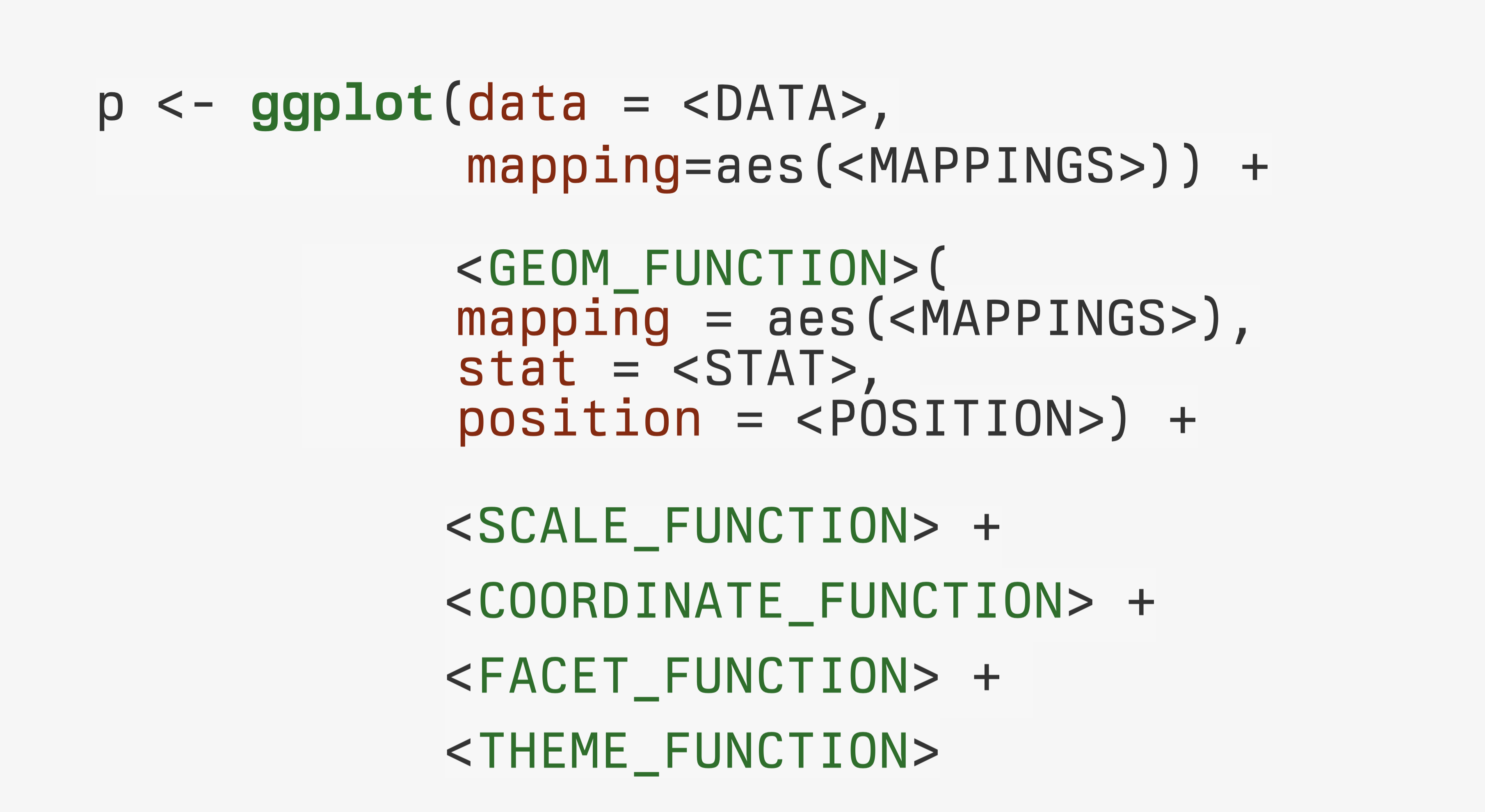
Core grammar
Grouped data; faceting
- Along with a few peeks at scale transformations, guide adjustments, and theme adjustment
All basic steps
dplyr and Pipelining
The elements of filtering and summarizing
gss_sm |>
group_by(bigregion, religion) |>
tally() |>
mutate(freq = n / sum(n),
pct = round((freq*100), 1)) # A tibble: 24 × 5
# Groups: bigregion [4]
bigregion religion n freq pct
<fct> <fct> <int> <dbl> <dbl>
1 Northeast Protestant 158 0.324 32.4
2 Northeast Catholic 162 0.332 33.2
3 Northeast Jewish 27 0.0553 5.5
4 Northeast None 112 0.230 23
5 Northeast Other 28 0.0574 5.7
6 Northeast <NA> 1 0.00205 0.2
7 Midwest Protestant 325 0.468 46.8
8 Midwest Catholic 172 0.247 24.7
9 Midwest Jewish 3 0.00432 0.4
10 Midwest None 157 0.226 22.6
# ℹ 14 more rowsExample and extension:
Organ Donation data
organdata is in the socviz package
# A tibble: 238 × 21
country year donors pop pop_dens gdp gdp_lag health health_lag
<chr> <date> <dbl> <int> <dbl> <int> <int> <dbl> <dbl>
1 Australia NA NA 17065 0.220 16774 16591 1300 1224
2 Australia 1991-01-01 12.1 17284 0.223 17171 16774 1379 1300
3 Australia 1992-01-01 12.4 17495 0.226 17914 17171 1455 1379
4 Australia 1993-01-01 12.5 17667 0.228 18883 17914 1540 1455
5 Australia 1994-01-01 10.2 17855 0.231 19849 18883 1626 1540
6 Australia 1995-01-01 10.2 18072 0.233 21079 19849 1737 1626
7 Australia 1996-01-01 10.6 18311 0.237 21923 21079 1846 1737
8 Australia 1997-01-01 10.3 18518 0.239 22961 21923 1948 1846
9 Australia 1998-01-01 10.5 18711 0.242 24148 22961 2077 1948
10 Australia 1999-01-01 8.67 18926 0.244 25445 24148 2231 2077
# ℹ 228 more rows
# ℹ 12 more variables: pubhealth <dbl>, roads <dbl>, cerebvas <int>,
# assault <int>, external <int>, txp_pop <dbl>, world <chr>, opt <chr>,
# consent_law <chr>, consent_practice <chr>, consistent <chr>, ccode <chr>First look

First look

First look

First look

First look

First look

Summarize better
with dplyr
Summarize a bunch of variables
by_country <- organdata |>
group_by(consent_law, country) |>
summarize(donors_mean= mean(donors, na.rm = TRUE),
donors_sd = sd(donors, na.rm = TRUE),
gdp_mean = mean(gdp, na.rm = TRUE),
health_mean = mean(health, na.rm = TRUE),
roads_mean = mean(roads, na.rm = TRUE),
cerebvas_mean = mean(cerebvas, na.rm = TRUE))
head(by_country)# A tibble: 6 × 8
# Groups: consent_law [1]
consent_law country donors_mean donors_sd gdp_mean health_mean roads_mean
<chr> <chr> <dbl> <dbl> <dbl> <dbl> <dbl>
1 Informed Australia 10.6 1.14 22179. 1958. 105.
2 Informed Canada 14.0 0.751 23711. 2272. 109.
3 Informed Denmark 13.1 1.47 23722. 2054. 102.
4 Informed Germany 13.0 0.611 22163. 2349. 113.
5 Informed Ireland 19.8 2.48 20824. 1480. 118.
6 Informed Netherlands 13.7 1.55 23013. 1993. 76.1
# ℹ 1 more variable: cerebvas_mean <dbl>- This works, but there’s so much repetition! It’s an open invitation to make mistakes copying and pasting.
DRY:
Don’t Repeat Yourself
Use across() and where() instead
by_country <- organdata |>
group_by(consent_law, country) |>
summarize(across(where(is.numeric),
list(mean = \(x) mean(x, na.rm = TRUE),
sd = \(x) sd(x, na.rm = TRUE))))
head(by_country) # A tibble: 6 × 28
# Groups: consent_law [1]
consent_law country donors_mean donors_sd pop_mean pop_sd pop_dens_mean
<chr> <chr> <dbl> <dbl> <dbl> <dbl> <dbl>
1 Informed Australia 10.6 1.14 18318. 831. 0.237
2 Informed Canada 14.0 0.751 29608. 1193. 0.297
3 Informed Denmark 13.1 1.47 5257. 80.6 12.2
4 Informed Germany 13.0 0.611 80255. 5158. 22.5
5 Informed Ireland 19.8 2.48 3674. 132. 5.23
6 Informed Netherlands 13.7 1.55 15548. 373. 37.4
# ℹ 21 more variables: pop_dens_sd <dbl>, gdp_mean <dbl>, gdp_sd <dbl>,
# gdp_lag_mean <dbl>, gdp_lag_sd <dbl>, health_mean <dbl>, health_sd <dbl>,
# health_lag_mean <dbl>, health_lag_sd <dbl>, pubhealth_mean <dbl>,
# pubhealth_sd <dbl>, roads_mean <dbl>, roads_sd <dbl>, cerebvas_mean <dbl>,
# cerebvas_sd <dbl>, assault_mean <dbl>, assault_sd <dbl>,
# external_mean <dbl>, external_sd <dbl>, txp_pop_mean <dbl>,
# txp_pop_sd <dbl>Use across() and where() instead
by_country <- organdata |>
group_by(consent_law, country) |>
summarize(across(where(is.numeric),
list(mean = \(x) mean(x, na.rm = TRUE),
sd = \(x) sd(x, na.rm = TRUE))),
.groups = "drop")
head(by_country) # A tibble: 6 × 28
consent_law country donors_mean donors_sd pop_mean pop_sd pop_dens_mean
<chr> <chr> <dbl> <dbl> <dbl> <dbl> <dbl>
1 Informed Australia 10.6 1.14 18318. 831. 0.237
2 Informed Canada 14.0 0.751 29608. 1193. 0.297
3 Informed Denmark 13.1 1.47 5257. 80.6 12.2
4 Informed Germany 13.0 0.611 80255. 5158. 22.5
5 Informed Ireland 19.8 2.48 3674. 132. 5.23
6 Informed Netherlands 13.7 1.55 15548. 373. 37.4
# ℹ 21 more variables: pop_dens_sd <dbl>, gdp_mean <dbl>, gdp_sd <dbl>,
# gdp_lag_mean <dbl>, gdp_lag_sd <dbl>, health_mean <dbl>, health_sd <dbl>,
# health_lag_mean <dbl>, health_lag_sd <dbl>, pubhealth_mean <dbl>,
# pubhealth_sd <dbl>, roads_mean <dbl>, roads_sd <dbl>, cerebvas_mean <dbl>,
# cerebvas_sd <dbl>, assault_mean <dbl>, assault_sd <dbl>,
# external_mean <dbl>, external_sd <dbl>, txp_pop_mean <dbl>,
# txp_pop_sd <dbl>Plot our summary data

What about faceting it instead?
The problem is that countries can only be in one Consent Law category.

What about faceting it instead?
Restricting to one column doesn’t fix it.

Allow the y-scale to vary
Normally the point of a facet is to preserve comparability between panels by not allowing the scales to vary. But for categorical measures it can be useful to allow this.

Again, these methods are general
by_country |>
ggplot(mapping =
aes(x = donors_mean,
y = reorder(country, donors_mean),
color = consent_law)) +
geom_pointrange(mapping =
aes(xmin = donors_mean - donors_sd,
xmax = donors_mean + donors_sd)) +
guides(color = "none") +
facet_wrap(~ consent_law,
ncol = 1,
scales = "free_y") +
labs(x = "Donor Procurement Rate",
y = NULL,
color = "Consent Law")
across() and where() again
# A tibble: 2,867 × 2
madeg padeg
<fct> <fct>
1 High School Graduate
2 High School Lt High School
3 Lt High School High School
4 High School <NA>
5 High School Bachelor
6 High School <NA>
7 High School High School
8 Lt High School Lt High School
9 Lt High School Lt High School
10 High School High School
# ℹ 2,857 more rowsacross() and where() again
gss_sm |>
group_by(sex, padeg) |>
summarize(across(where(is.numeric),
list(mean = ~ mean(.x, na.rm = TRUE),
sd = ~ sd(.x, na.rm = TRUE)))) |>
select(sex, padeg, contains(c("age", "childs", "sibs"))) # A tibble: 12 × 8
# Groups: sex [2]
sex padeg age_mean age_sd childs_mean childs_sd sibs_mean sibs_sd
<fct> <fct> <dbl> <dbl> <dbl> <dbl> <dbl> <dbl>
1 Male Lt High School 57.8 16.8 2.54 2.06 4.86 3.46
2 Male High School 46.7 16.7 1.54 1.52 3.14 2.76
3 Male Junior College 39.9 16.9 1.07 1.44 3.30 2.87
4 Male Bachelor 43.3 14.6 1.27 1.35 2.54 2.41
5 Male Graduate 39.9 14.8 1.01 1.35 2.36 1.88
6 Male <NA> 47.1 17.1 1.75 1.67 3.84 3.21
7 Female Lt High School 58.5 18.0 2.46 1.72 4.74 3.43
8 Female High School 48.5 17.4 1.76 1.48 3.12 2.82
9 Female Junior College 39.2 11.6 1.46 1.43 3.19 2.00
10 Female Bachelor 44.8 15.4 1.32 1.35 2.88 2.62
11 Female Graduate 43.5 13.8 1.42 1.26 2.33 1.50
12 Female <NA> 47.4 17.8 2.08 1.69 4.65 3.93across() and where() again
gss_sm |>
select(padeg, madeg, contains(c("age", "childs", "sibs"))) |>
group_by(padeg, madeg) |>
summarize(across(where(is.numeric),
list(
mean = \(x) mean(x, na.rm = TRUE),
sd = \(x) sd(x, na.rm = TRUE)
))) |>
drop_na() |>
ggplot(mapping = aes(x = childs_mean,
xmin = childs_mean - childs_sd,
xmax = childs_mean + childs_sd,
y = madeg)) +
geom_pointrange() +
facet_wrap(~ padeg, ncol = 5)
Dogs of New York again
# A tibble: 493,072 × 9
   animal_name animal_gender animal_birth_year breed_rc         borough zip_code
   <chr>       <chr>                     <dbl> <chr>            <chr>      <int>
 1 Paige       F                          2014 Pit Bull (or Mi… Manhat…    10035
 2 Yogi        M                          2010 Boxer            Bronx      10465
 3 Ali         M                          2014 Basenji          Manhat…    10013
 4 Queen       F                          2013 Akita Crossbreed Manhat…    10013
 5 Lola        F                          2009 Maltese          Manhat…    10028
 6 Ian         M                          2006 Unknown          Manhat…    10013
 7 Buddy       M                          2008 Unknown          Manhat…    10025
 8 Chewbacca   F                          2012 Labrador (or Cr… Manhat…    10013
 9 Heidi-Bo    F                          2007 Dachshund Smoot… Brookl…    11215
10 Massimo     M                          2009 Bull Dog, French Brookl…    11201
# ℹ 493,062 more rows
# ℹ 3 more variables: license_issued_date <date>, license_expired_date <date>,
# extract_year <dbl>arrange() and slice()
arrange() and slice()
arrange() and slice()
arrange() and slice()
# A tibble: 327 × 2
   breed_rc                       n
   <chr>                      <int>
 1 Affenpinscher                136
 2 Afghan Hound                  89
 3 Afghan Hound Crossbreed       19
 4 Airedale Terrier             227
 5 Akita                        491
 6 Akita Crossbreed             151
 7 Alaskan Klee Kai             113
 8 Alaskan Malamute             287
 9 American Bully              1100
10 American English Coonhound   103
# ℹ 317 more rows
arrange() and slice()
# A tibble: 327 × 2
   breed_rc                     n
   <chr>                    <int>
 1 Unknown                  54586
 2 Yorkshire Terrier        30379
 3 Labrador (or Crossbreed) 28399
 4 Shih Tzu                 27407
 5 Pit Bull (or Mix)        24393
 6 Chihuahua                21211
 7 Maltese                  15701
 8 Pomeranian                9287
 9 Havanese                  8606
10 Shih Tzu Crossbreed       8098
# ℹ 317 more rows
arrange() and slice()
arrange() and slice()
nyc_license |>
  group_by(borough, breed_rc) |>
  drop_na() |>
  tally() |>
  slice_max(order_by = n,
            n = 5)
# A tibble: 25 × 3
# Groups: borough [5]
borough breed_rc n
<chr> <chr> <int>
1 Bronx Yorkshire Terrier 3583
2 Bronx Pit Bull (or Mix) 3517
3 Bronx Unknown 3484
4 Bronx Shih Tzu 2970
5 Bronx Chihuahua 2224
6 Brooklyn Unknown 9707
7 Brooklyn Yorkshire Terrier 5736
8 Brooklyn Pit Bull (or Mix) 5538
9 Brooklyn Shih Tzu 5281
10 Brooklyn Labrador (or Crossbreed) 5179
# ℹ 15 more rowsarrange() and slice()
nyc_license |>
  group_by(borough, breed_rc) |>
  drop_na() |>
  tally() |>
  slice_max(order_by = n,
            prop = 0.05)
# A tibble: 64 × 3
# Groups: borough [5]
borough breed_rc n
<chr> <chr> <int>
1 Bronx Yorkshire Terrier 3583
2 Bronx Pit Bull (or Mix) 3517
3 Bronx Unknown 3484
4 Bronx Shih Tzu 2970
5 Bronx Chihuahua 2224
6 Bronx Maltese 1382
7 Bronx Labrador (or Crossbreed) 1340
8 Bronx Shih Tzu Crossbreed 819
9 Bronx Pomeranian 667
10 Bronx Chihuahua Crossbreed 638
# ℹ 54 more rows