library(here)       # manage file paths
library(socviz)     # data and some useful things, especially %nin%
library(tidyverse)  # your friend and mine

library(scales)     # Convenient scale labels

## New packages
# install.packages("tsibble") # Time series objects
# install.packages("feasts")  # Time series feature analysis
# install.packages("slider")  # Moving averages and related methods
# remotes::install_github("kjhealy/demog") # Some US demographic data

library(tsibble)
library(feasts)
library(slider)
library(demog)08 — Change over Time
Kieran Healy
March 1, 2024
Change over
Time
Load our libraries
A Time Series: US Monthly Births
boom <- okboomer |>
  filter(country == "United States") |>
  select(date, total_pop, births_pct_day) |>
  rename(births = births_pct_day)

boom
# A tibble: 996 × 3
date total_pop births
<date> <dbl> <dbl>
1 1933-01-01 125579000 46.4
2 1933-02-01 125579000 47.2
3 1933-03-01 125579000 47.2
4 1933-04-01 125579000 45.5
5 1933-05-01 125579000 44.9
6 1933-06-01 125579000 44.9
7 1933-07-01 125579000 46.5
8 1933-08-01 125579000 46.7
9 1933-09-01 125579000 44.5
10 1933-10-01 125579000 42.9
# ℹ 986 more rowsHere the births column means “Average daily births per million population”
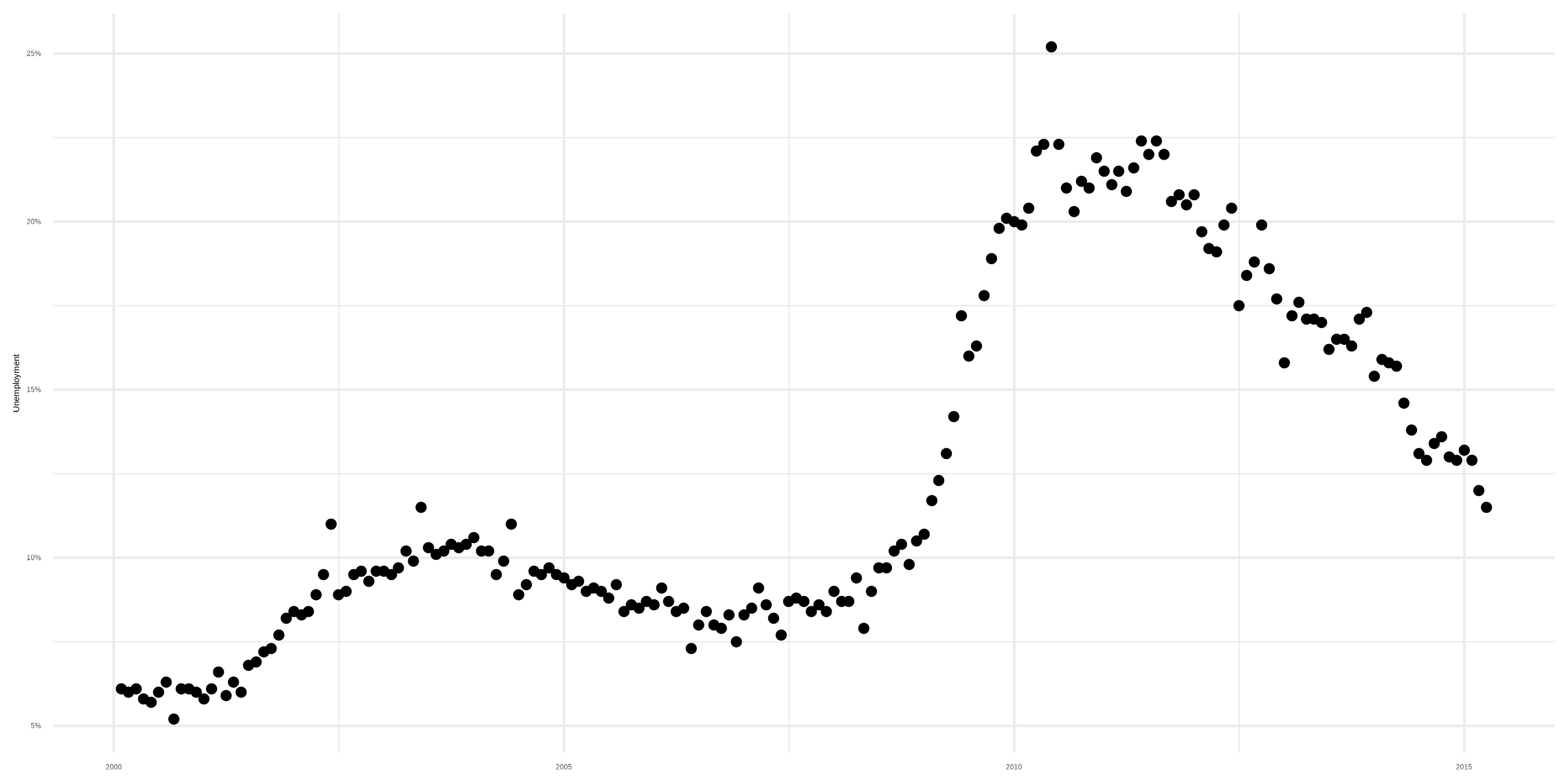
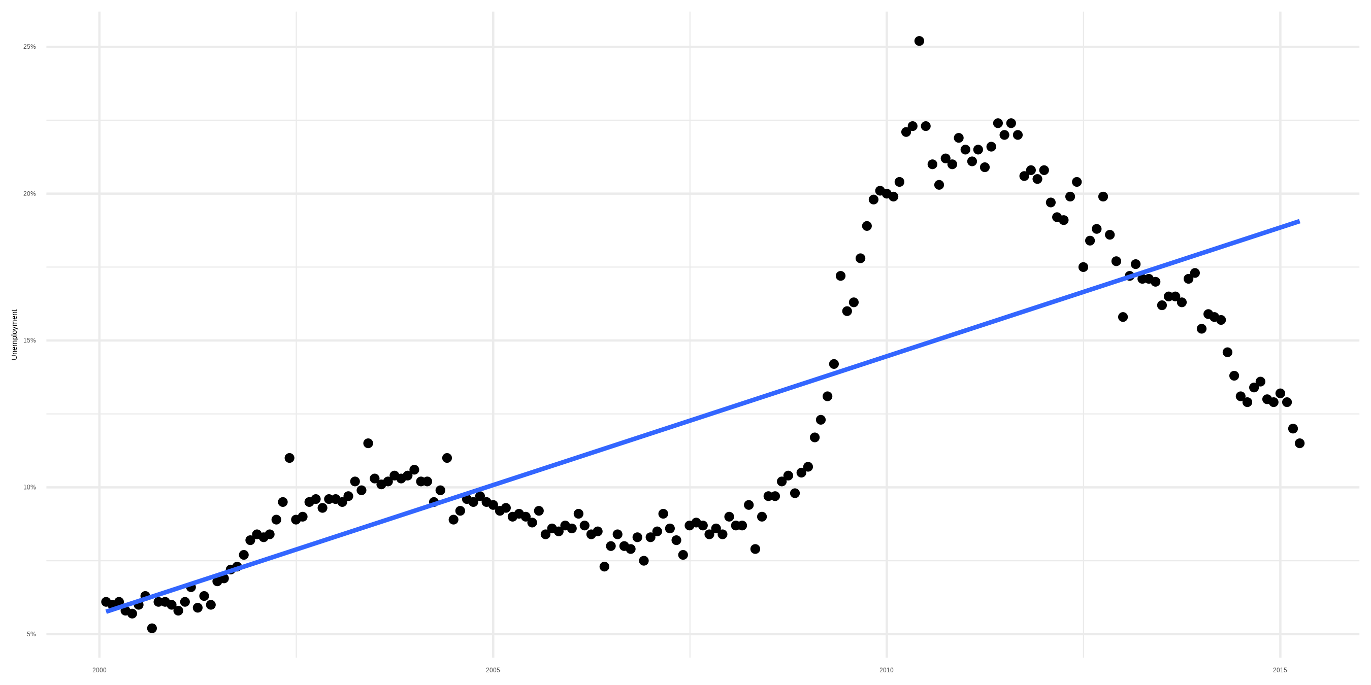
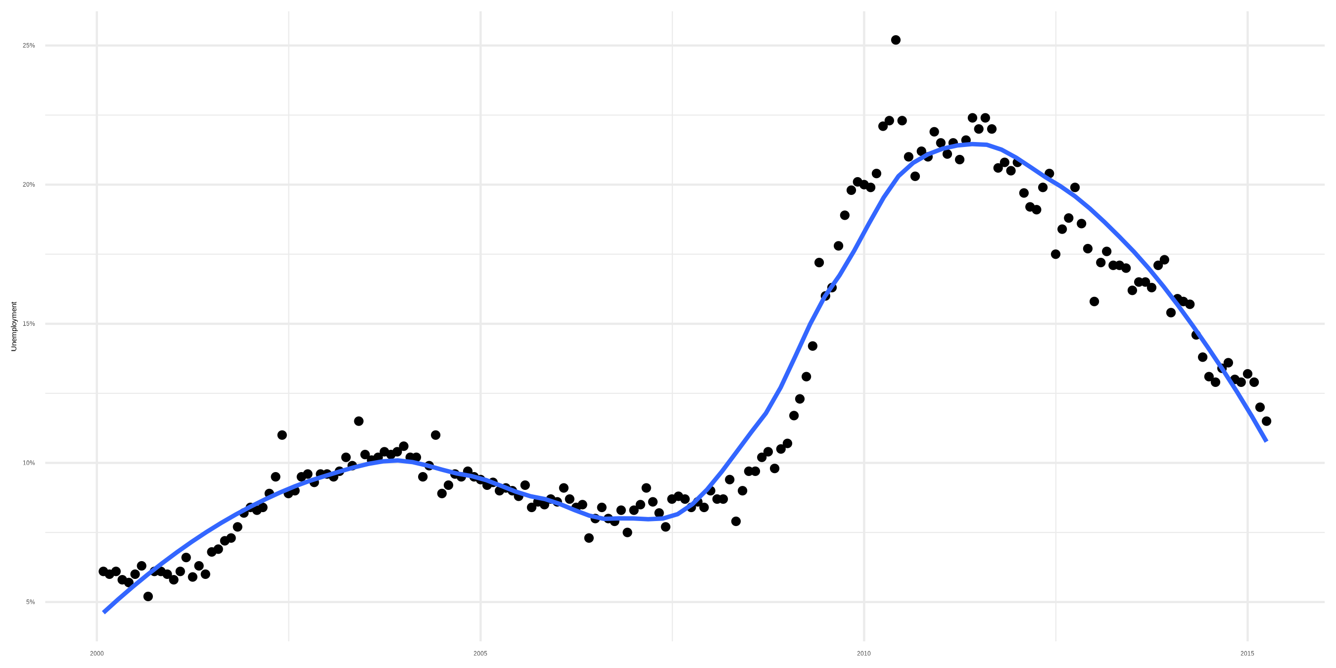
Looking at the Series

Looking at the Series

Too much smoothing here
Time Series Decomposition
The analysis of Time Series is a big area; people often want to see into the future
We will focus on a couple of elementary methods that are more purely descriptive, particularly the idea of decomposing a time series into its trend, seasonal, and remainder components.
Decomposition methods are descriptive rather than predictive. They also make assumptions about the character of the data (e.g. its seasonality) which might be something we want to investigate.
More complex forecasting methods are either more detailed, or attempt to be proper models, or both.
Centered Moving Averages: slider
# A tibble: 996 × 4
   date       total_pop births   ma3
   <date>         <dbl>  <dbl> <dbl>
 1 1933-01-01 125579000   46.4  NA
 2 1933-02-01 125579000   47.2  46.9
 3 1933-03-01 125579000   47.2  46.6
 4 1933-04-01 125579000   45.5  45.9
 5 1933-05-01 125579000   44.9  45.1
 6 1933-06-01 125579000   44.9  45.4
 7 1933-07-01 125579000   46.5  46.0
 8 1933-08-01 125579000   46.7  45.9
 9 1933-09-01 125579000   44.5  44.7
10 1933-10-01 125579000   42.9  43.8
# ℹ 986 more rows
Centered Moving Averages: slider
Centered Moving Averages: slider

A Centered Moving Average, order 5
A Centered Moving Average, order 5

A Centered Moving Average, order 7
As the order goes up, the window for the average widens, and the line gets smoother and smoother.
A Centered Moving Average, order 7

Odd vs Even Centering
Even orders have to be calculated differently
When the period \(m\) is odd, the average \(d\) for an observation \(y\) at a particular time \(t\) is:
\[\begin{equation} d_t = \frac{1}{m}\sum_{i=-(m-1)/2}^{(m-1)/2} y_{t+i} \end{equation}\]
Odd vs Even Centering
When the period is even, it’s:
\[\begin{equation} d_t = \frac{1}{m}\left(\frac{1}{2}\left(y_{t+(m-1)/2}+y_{t-(m-1)/2}\right) + \sum_{i=-(m-2)/2}^{(m-2)/2} y_{t+i}\right) \end{equation}\]
This just means e.g. we use half of December of the previous year and half of December of the current year to calculate the centred moving average in June of the current year.
A Centered Moving Average of order 12
We can calculate the CMA for even orders in two steps.
boom |>
  mutate(
    mav12 = slide_dbl(births, mean,
                    .before = 5, .after = 6,
                    .complete = TRUE),
    mav2x12 = slide_dbl(mav12, mean,
                         .before = 1, .after = 0,
                         .complete = TRUE))
# A tibble: 996 × 5
date total_pop births mav12 mav2x12
<date> <dbl> <dbl> <dbl> <dbl>
1 1933-01-01 125579000 46.4 NA NA
2 1933-02-01 125579000 47.2 NA NA
3 1933-03-01 125579000 47.2 NA NA
4 1933-04-01 125579000 45.5 NA NA
5 1933-05-01 125579000 44.9 NA NA
6 1933-06-01 125579000 44.9 45.4 NA
7 1933-07-01 125579000 46.5 45.4 45.4
8 1933-08-01 125579000 46.7 45.4 45.4
9 1933-09-01 125579000 44.5 45.3 45.4
10 1933-10-01 125579000 42.9 45.2 45.3
# ℹ 986 more rowsSee how we lose observations as our window widens.
A Centered Moving Average, order 12
boom |>
  mutate(
    mav12 = slide_dbl(births, mean,
                    .before = 5, .after = 6,
                    .complete = TRUE),
    mav2x12 = slide_dbl(mav12, mean,
                         .before = 1, .after = 0,
                         .complete = TRUE)) |>
  ggplot() +
  geom_line(aes(x = date, y = births)) +
  geom_line(aes(x = date, y = mav2x12), linewidth = rel(1.2), color = "firebrick") +
labs(title = "12 month moving average")A Centered Moving Average, order 12

A 5 year CMA
boom |>
  mutate(
    mav12 = slide_dbl(births, mean,
                    .before = 29, .after = 30,
                    .complete = TRUE),
    mav2x12 = slide_dbl(mav12, mean,
                         .before = 1, .after = 0,
                         .complete = TRUE)) |>
  ggplot() +
  geom_line(aes(x = date, y = births)) +
  geom_line(aes(x = date, y = mav2x12), linewidth = rel(1.2), color = "firebrick") +
labs(title = "5 year moving average")A 5 year CMA

Seasonality in US Birth Rates
Seasonality in US Birth Rates

The Additive “Classical” Decomposition
The Thing to be Decomposed: the births series, \(y\)
A Trend Part: a centered moving average, \(\hat{T}\)
A Seasonal Part: the “pulse” in the data, \(\hat{S}\)
A Remainder Part: the leftover part, \(\hat{R}\)
The trend \(y\) is then \(y = \hat{T} + \hat{S} + \hat{R}\)
Calculate the Trend part
This is the moving average we just calculated.
boom_t <- boom |>
  select(date, births) |>
  mutate(
    month = lubridate::month(date),
    mav12 = slide_dbl(births, mean, .before = 5, .after = 6,
                    .complete = TRUE),
    t = slide_dbl(mav12, mean, .before = 1, .after = 0,
                         .complete = TRUE)) |>
  select(-mav12) # Don't need this anymore
boom_t
# A tibble: 996 × 4
date births month t
<date> <dbl> <dbl> <dbl>
1 1933-01-01 46.4 1 NA
2 1933-02-01 47.2 2 NA
3 1933-03-01 47.2 3 NA
4 1933-04-01 45.5 4 NA
5 1933-05-01 44.9 5 NA
6 1933-06-01 44.9 6 NA
7 1933-07-01 46.5 7 45.4
8 1933-08-01 46.7 8 45.4
9 1933-09-01 44.5 9 45.4
10 1933-10-01 42.9 10 45.3
# ℹ 986 more rowsCalculate the Seasonal part
First “detrend” the series by subtracting t from births.
# A tibble: 996 × 5
date births month t detrended
<date> <dbl> <dbl> <dbl> <dbl>
1 1933-01-01 46.4 1 NA NA
2 1933-02-01 47.2 2 NA NA
3 1933-03-01 47.2 3 NA NA
4 1933-04-01 45.5 4 NA NA
5 1933-05-01 44.9 5 NA NA
6 1933-06-01 44.9 6 NA NA
7 1933-07-01 46.5 7 45.4 1.04
8 1933-08-01 46.7 8 45.4 1.29
9 1933-09-01 44.5 9 45.4 -0.861
10 1933-10-01 42.9 10 45.3 -2.34
# ℹ 986 more rowsCalculate the Seasonal part
Then take the average by month.
boom_t |>
mutate(detrended = births - t,
month = lubridate::month(date)) |>
group_by(month) |>
summarize(seasonal = mean(detrended, na.rm = TRUE))# A tibble: 12 × 2
month seasonal
<dbl> <dbl>
1 1 -1.62
2 2 -0.578
3 3 -0.912
4 4 -2.21
5 5 -1.99
6 6 -0.333
7 7 1.90
8 8 2.74
9 9 3.39
10 10 0.765
11 11 -0.564
12 12 -0.625Calculate the Seasonal part
Then “mean-center” each point by taking the average again and subtracting it from each observation. (This way the observations all sum to zero.)
boom_t |>
mutate(detrended = births - t) |>
group_by(month) |>
summarize(sm = mean(detrended, na.rm = TRUE)) |>
mutate(s = sm - mean(sm)) # A tibble: 12 × 3
month sm s
<dbl> <dbl> <dbl>
1 1 -1.62 -1.62
2 2 -0.578 -0.575
3 3 -0.912 -0.909
4 4 -2.21 -2.21
5 5 -1.99 -1.98
6 6 -0.333 -0.330
7 7 1.90 1.90
8 8 2.74 2.74
9 9 3.39 3.40
10 10 0.765 0.768
11 11 -0.564 -0.561
12 12 -0.625 -0.622Calculate the Seasonal part
- Put this in an object
boom_s <- boom_t |>
  mutate(detrended = births - t) |>
  group_by(month) |>
  summarize(sm = mean(detrended, na.rm = TRUE)) |>
  mutate(s = sm - mean(sm)) |>
  select(-sm) # don't need this anymore

boom_s
# A tibble: 12 × 2
month s
<dbl> <dbl>
1 1 -1.62
2 2 -0.575
3 3 -0.909
4 4 -2.21
5 5 -1.98
6 6 -0.330
7 7 1.90
8 8 2.74
9 9 3.40
10 10 0.768
11 11 -0.561
12 12 -0.622Calculate the Seasonal part
Join it to the main table
# A tibble: 996 × 5
   date       births month     t      s
   <date>      <dbl> <dbl> <dbl>  <dbl>
 1 1933-01-01   46.4     1  NA   -1.62
 2 1933-02-01   47.2     2  NA   -0.575
 3 1933-03-01   47.2     3  NA   -0.909
 4 1933-04-01   45.5     4  NA   -2.21
 5 1933-05-01   44.9     5  NA   -1.98
 6 1933-06-01   44.9     6  NA   -0.330
 7 1933-07-01   46.5     7  45.4  1.90
 8 1933-08-01   46.7     8  45.4  2.74
 9 1933-09-01   44.5     9  45.4  3.40
10 1933-10-01   42.9    10  45.3  0.768
# ℹ 986 more rows
Calculate the Seasonal part
In a “Classical” decomposition the Seasonal part just repeats.

Calculate the Remainder part
The remainder is just what’s left over from y (i.e., births) after we have calculated t and s.
# A tibble: 996 × 6
   date       births month     t      s      r
   <date>      <dbl> <dbl> <dbl>  <dbl>  <dbl>
 1 1933-01-01   46.4     1  NA   -1.62  NA
 2 1933-02-01   47.2     2  NA   -0.575 NA
 3 1933-03-01   47.2     3  NA   -0.909 NA
 4 1933-04-01   45.5     4  NA   -2.21  NA
 5 1933-05-01   44.9     5  NA   -1.98  NA
 6 1933-06-01   44.9     6  NA   -0.330 NA
 7 1933-07-01   46.5     7  45.4  1.90  -0.863
 8 1933-08-01   46.7     8  45.4  2.74  -1.46
 9 1933-09-01   44.5     9  45.4  3.40  -4.26
10 1933-10-01   42.9    10  45.3  0.768 -3.11
# ℹ 986 more rows
Decomposition: y = t + s + r
This is an additive decomposition. You can also do multiplicative decompositions.
# A tibble: 996 × 7
   date       births month     t      s      r   tsr
   <date>      <dbl> <dbl> <dbl>  <dbl>  <dbl> <dbl>
 1 1933-01-01   46.4     1  NA   -1.62  NA      NA
 2 1933-02-01   47.2     2  NA   -0.575 NA      NA
 3 1933-03-01   47.2     3  NA   -0.909 NA      NA
 4 1933-04-01   45.5     4  NA   -2.21  NA      NA
 5 1933-05-01   44.9     5  NA   -1.98  NA      NA
 6 1933-06-01   44.9     6  NA   -0.330 NA      NA
 7 1933-07-01   46.5     7  45.4  1.90  -0.863  46.5
 8 1933-08-01   46.7     8  45.4  2.74  -1.46   46.7
 9 1933-09-01   44.5     9  45.4  3.40  -4.26   44.5
10 1933-10-01   42.9    10  45.3  0.768 -3.11   42.9
# ℹ 986 more rows
There’s no need to it manually
boom |>
  mutate(date = yearmonth(date)) |>
  as_tsibble(index = "date") |>
  model(
    classical_decomposition(births,
                            type = "additive")
  ) |>
  components() |>
  select(-.model)
# A tsibble: 996 x 6 [1M]
date births trend seasonal random season_adjust
<mth> <dbl> <dbl> <dbl> <dbl> <dbl>
1 1933 Jan 46.4 NA -1.62 NA 48.0
2 1933 Feb 47.2 NA -0.575 NA 47.8
3 1933 Mar 47.2 NA -0.909 NA 48.1
4 1933 Apr 45.5 NA -2.21 NA 47.7
5 1933 May 44.9 NA -1.98 NA 46.9
6 1933 Jun 44.9 NA -0.330 NA 45.3
7 1933 Jul 46.5 45.4 1.90 -0.863 44.6
8 1933 Aug 46.7 45.4 2.74 -1.46 44.0
9 1933 Sep 44.5 45.4 3.40 -4.26 41.1
10 1933 Oct 42.9 45.3 0.768 -3.11 42.1
# ℹ 986 more rowsPlot all the components at once
Plot all the components at once

The STL Decomposition
More robust and flexible than Classical Decomposition
Due to William Cleveland
Uses LOESS, a little like geom_smooth()
Good for monthly and annual data
You have to choose the Trend and Seasonal Windows
Sidenote: Smoothers
A trend
Sidenote: Smoothers
Smoother with bad linear fit
Sidenote: Smoothers
Smoother with loess fit
Sidenote: Smoothers
Sidenote: Smoothers
The STL Decomposition
Default seasonal monthly window is 13
This works for monthly data
Default monthly trend window is 21
You can experiment with these
They should be odd numbers
The STL Decomposition
The STL Decomposition

Manually plotting the components
bc <- boom |>
  mutate(date = yearmonth(date)) |>
  as_tsibble(index = "date") |>
  model(
    # Experiment with a six-monthly trend window
    STL(births ~ trend(window = 7) +
          season(window = 7),
        robust = TRUE)
  ) |>
  components() |>
  select(-.model)

bc
# A tsibble: 996 x 6 [1M]
date births trend season_year remainder season_adjust
<mth> <dbl> <dbl> <dbl> <dbl> <dbl>
1 1933 Jan 46.4 46.4 -0.148 0.0757 46.5
2 1933 Feb 47.2 46.4 0.969 -0.197 46.2
3 1933 Mar 47.2 46.4 0.781 0.0247 46.4
4 1933 Apr 45.5 46.3 -1.17 0.304 46.7
5 1933 May 44.9 46.1 -1.49 0.329 46.4
6 1933 Jun 44.9 45.5 -0.646 0.0632 45.6
7 1933 Jul 46.5 44.8 2.25 -0.632 44.2
8 1933 Aug 46.7 44.6 2.40 -0.278 44.3
9 1933 Sep 44.5 45.0 2.47 -2.98 42.0
10 1933 Oct 42.9 45.6 -0.584 -2.12 43.5
# ℹ 986 more rowsManually plotting the components
bc |>
  pivot_longer(cols = c(births, trend, season_year, remainder)) |>
  mutate(
    date = as.Date(date),
    name = factor(name, levels = c("births", "trend",
                                        "season_year", "remainder"),
                  labels = c("Births", "Trend", "Seasonal", "Remainder"),
                       ordered = TRUE)) |>
  ggplot() +
  geom_line(aes(date, value)) +
  scale_x_date(breaks = seq(as.Date("1935-01-01"),
                                 as.Date("2015-01-01"),
                                 by="10 years"),
               date_labels = "%Y") +
  ggforce::facet_col(~ name, scales = 'free', space = 'free') +
  labs(title = "Decomposition of US Monthly Births, 1933-2017",
       subtitle = "Average number of daily births per million population each month",
       x = "Time", y = "Birth rate")
Manually plotting the components

Comparing seasonality
s30s <- lubridate::interval(ymd(19330101), ymd(19390101))
s50s <- lubridate::interval(ymd(19530101), ymd(19590101))
s00s <- lubridate::interval(ymd(20030101), ymd(20090101))

my_intervs <- list(s30s, s50s, s00s)

bc_int <- bc |>
  mutate(date = as.Date(date)) |>
  filter(date %within% my_intervs) |>
  mutate(period = case_when(
    date %within% s30s ~ "1930s",
    date %within% s50s ~ "1950s",
    date %within% s00s ~ "2000s"),
    year = year(date),
    month = month(date, label = TRUE,
                  abbr = TRUE)) |>
  mutate(yr_id = consecutive_id(year), .by = period) |>
  mutate(mth_id = row_number(), .by = c(period, year)) |>
  mutate(seq_id = row_number(), .by = period)
Comparing seasonality
# A tsibble: 219 x 12 [1D]
   date       births trend season_year remainder season_adjust period  year
   <date>      <dbl> <dbl>       <dbl>     <dbl>         <dbl> <chr>  <dbl>
 1 1933-01-01   46.4  46.4      -0.148    0.0757          46.5 1930s   1933
 2 1933-02-01   47.2  46.4       0.969   -0.197           46.2 1930s   1933
 3 1933-03-01   47.2  46.4       0.781    0.0247          46.4 1930s   1933
 4 1933-04-01   45.5  46.3      -1.17     0.304           46.7 1930s   1933
 5 1933-05-01   44.9  46.1      -1.49     0.329           46.4 1930s   1933
 6 1933-06-01   44.9  45.5      -0.646    0.0632          45.6 1930s   1933
 7 1933-07-01   46.5  44.8       2.25    -0.632           44.2 1930s   1933
 8 1933-08-01   46.7  44.6       2.40    -0.278           44.3 1930s   1933
 9 1933-09-01   44.5  45.0       2.47    -2.98            42.0 1930s   1933
10 1933-10-01   42.9  45.6      -0.584   -2.12            43.5 1930s   1933
11 1933-11-01   44.0  46.6      -2.24    -0.298           46.3 1930s   1933
12 1933-12-01   44.2  46.6      -2.60     0.247           46.8 1930s   1933
13 1934-01-01   46.6  46.5      -0.159    0.272           46.8 1930s   1934
14 1934-02-01   47.0  46.2       0.988   -0.167           46.1 1930s   1934
15 1934-03-01   45.7  45.9       0.791   -0.984           44.9 1930s   1934
16 1934-04-01   44.5  46.1      -1.17    -0.397           45.7 1930s   1934
17 1934-05-01   45.7  46.4      -1.50     0.834           47.2 1930s   1934
18 1934-06-01   46.2  46.7      -0.668    0.0981          46.8 1930s   1934
19 1934-07-01   47.9  47.2       2.26    -1.53            45.7 1930s   1934
20 1934-08-01   49.9  47.6       2.43    -0.193           47.4 1930s   1934
# ℹ 199 more rows
# ℹ 4 more variables: month <ord>, yr_id <int>, mth_id <int>, seq_id <int>
Comparing seasonality
my_labs <- bc_int$seq_id
names(my_labs) <- bc_int$month

ind <- names(my_labs) %in% c("Jan", "May", "Sep")

my_labs <- my_labs[ind]

bc_int |>
  ggplot(aes(x = seq_id,
             y = season_year,
             color = period)) +
  geom_line(linewidth = rel(1.2)) +
  scale_x_continuous(breaks = my_labs,
                     labels = names(my_labs)) +
  facet_wrap(~ period, ncol = 1) +
  guides(color = "none") +
  labs(x = "Month",  y = "Seasonal Component of the Birth Rate",
       title = "Changing Seasonality in Births: Three Six-Year periods in Three Decades",
       subtitle = "Seasonal Component from an STL decomposition of 1933-2015 monthly births")
Comparing seasonality
