Example 02: Writing R Code

This week we are going to jump into writing R code. I encourage you to experiment and try things. As we go, we will develop a good working understanding of how R works. But the best way to make this happen is to just start doing things and talk about them as we go.

When starting an R work session, we typically load the packages we will need. This is like taking a book off your shelf to refer to. We only need to do this once per session.

library(tidyverse)

For now, don’t worry about any messages or warnings you get. But read them and think about what they are trying to tell you.

R basics

How do we write in R? How do we make it do things?

To start, we can say: in R, everything has a name and everything is an object. You do things to named objects with functions (which are themselves objects!). And you create an object by assigning a thing to a name.

Assignment is the act of attaching a thing to a name. It is represented by <- or = and you can read it as “gets” or “is”. Type it by with the < and then the - key. Better, there is a shortcut: on Mac OS it is Option - or Option and the - (minus or hyphen) key together. On Windows it’s Alt -.

Objects

We’re going to use the c() function (c for concatenate) to stick some numbers together into a vector. And we will assign that the name my_numbers.

## Inside code chunks, lines beginning with a # character are comments
## Comments are ignored by R

my_numbers <- c(1, 1, 2, 4, 1, 3, 1, 5) # Anything after a # character is ignored as well

## Now we have an object by this name
my_numbers 

[1] 1 1 2 4 1 3 1 5

Again, in that previous chunk we created an object by assigning something (the result of a function) to a name. Now that thing exists in our project environment.

my_numbers

[1] 1 1 2 4 1 3 1 5

R has a few built-in objects.

letters

 [1] "a" "b" "c" "d" "e" "f" "g" "h" "i" "j" "k" "l" "m" "n" "o" "p" "q" "r" "s"
[20] "t" "u" "v" "w" "x" "y" "z"

LETTERS

 [1] "A" "B" "C" "D" "E" "F" "G" "H" "I" "J" "K" "L" "M" "N" "O" "P" "Q" "R" "S"
[20] "T" "U" "V" "W" "X" "Y" "Z"

pi

[1] 3.141593

But mostly we will be creating objects.

R is a calculator

You don’t have to make objects. You can just treat R like a calculator that spits out answers at the console.

(31 * 12) / 2^4

[1] 23.25

sqrt(25)

[1] 5

log(100)

[1] 4.60517

log10(100)

[1] 2

The commands that look like this() are called functions.

But everything you do along these lines can, if you want, be assigned to a name. Like my_five <- sqrt(25).

You can do logic

4 < 10

[1] TRUE

4 > 2 & 1 > 0.5 # The "&" means "and"

[1] TRUE

4 < 2 | 1 > 0.5 # The "|" means "or"

[1] TRUE

4 < 2 | 1 < 0.5

[1] FALSE

A logical test:

2 == 2 # Write `=` twice

[1] TRUE

Not this:

## This will cause an error, because R will think you are trying to assign a value
2 = 2

## Error in 2 = 2 : invalid (do_set) left-hand side to assignment

Testing for “not equal to” or “is not”:

3 != 7 # Write `!` and then `=` to make `!=`

[1] TRUE

More about objects

my_numbers # We created this a few minutes ago

[1] 1 1 2 4 1 3 1 5

letters  # This one is built-in

 [1] "a" "b" "c" "d" "e" "f" "g" "h" "i" "j" "k" "l" "m" "n" "o" "p" "q" "r" "s"
[20] "t" "u" "v" "w" "x" "y" "z"

pi  # Also built-in

[1] 3.141593

Creating objects: assign a thing (usually the result of a function) to a name.

## this object... gets ... the output of this function
my_numbers <- c(1, 2, 3, 1, 3, 5, 25, 10)

your_numbers <- c(5, 31, 71, 1, 3, 21, 6, 52)

You do things with functions

Functions usually take input, perform actions, and then return output.

# Calculate the mean of my_numbers with the mean() function
mean(x = my_numbers)

[1] 6.25

The instructions you can give a function are its arguments. Here, x is saying “this is the thing I want you to take the mean of”.

If you provide arguments in the “right” order (the order the function expects), you don’t have to name them.

mean(my_numbers)

[1] 6.25

Look at the help for mean() with ?mean to learn what trim is doing.

## The sample() function 
x <- sample(x = 1:100, size = 100, replace = TRUE) # What does each piece do here?
mean(x)

[1] 47.38

mean(x, trim = 0.1) 

[1] 46.825

For functions with more than one or two arguments, explicitly naming arguments is good practice, especially when learning the language.

Data

A few datasets come built-in, for convenience. Here is one:

mpg

# A tibble: 234 × 11
   manufacturer model      displ  year   cyl trans drv     cty   hwy fl    class
   <chr>        <chr>      <dbl> <int> <int> <chr> <chr> <int> <int> <chr> <chr>
 1 audi         a4           1.8  1999     4 auto… f        18    29 p     comp…
 2 audi         a4           1.8  1999     4 manu… f        21    29 p     comp…
 3 audi         a4           2    2008     4 manu… f        20    31 p     comp…
 4 audi         a4           2    2008     4 auto… f        21    30 p     comp…
 5 audi         a4           2.8  1999     6 auto… f        16    26 p     comp…
 6 audi         a4           2.8  1999     6 manu… f        18    26 p     comp…
 7 audi         a4           3.1  2008     6 auto… f        18    27 p     comp…
 8 audi         a4 quattro   1.8  1999     4 manu… 4        18    26 p     comp…
 9 audi         a4 quattro   1.8  1999     4 auto… 4        16    25 p     comp…
10 audi         a4 quattro   2    2008     4 manu… 4        20    28 p     comp…
# ℹ 224 more rows

Graphs

To draw a graph in ggplot requires two kinds of statements: one saying what the data is and what relationship we want to plot, and the second saying what kind of plot we want.

The first one is done by the ggplot() function.

ggplot(data = mpg, 
       mapping = aes(x = displ, y = hwy))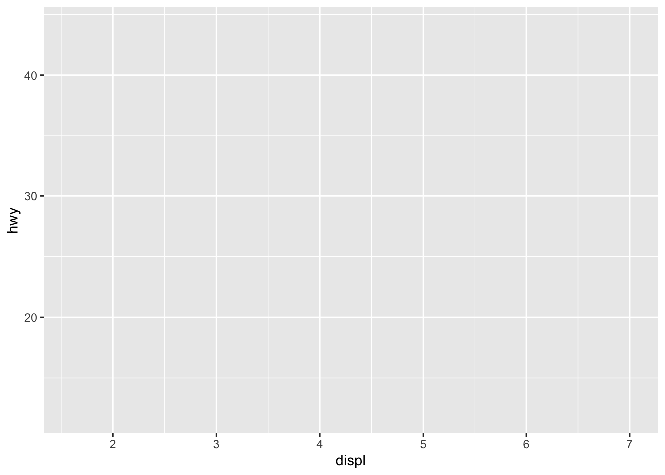

You can see that by itself it doesn’t do anything.

But if we add a function saying what kind of plot, we get a result:

ggplot(data = mpg, 
       mapping = aes(x = displ, y = hwy)) +
  geom_point()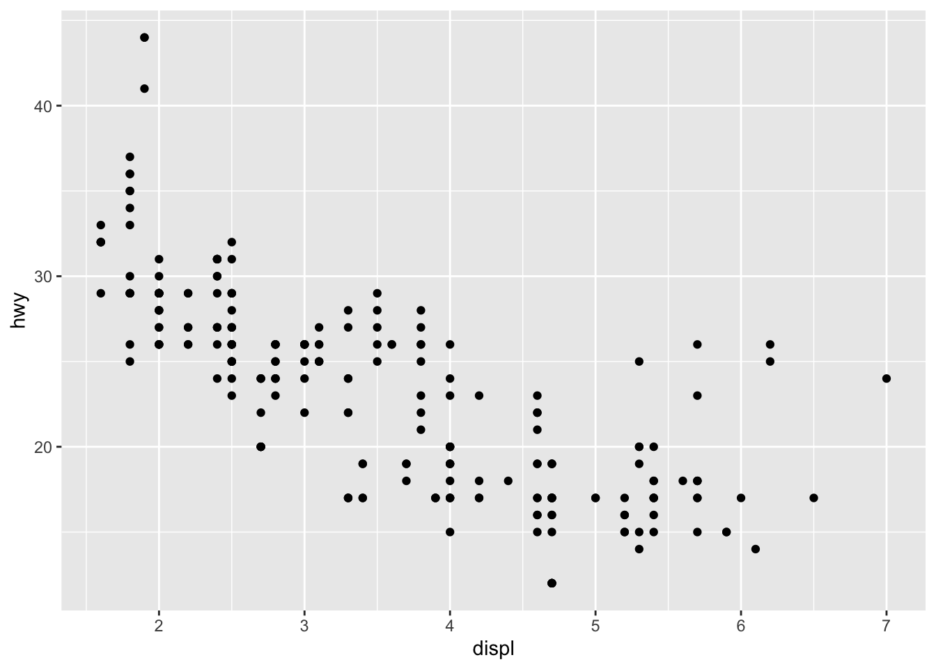

At this stage, a lot of this may seem obscure. What is a mapping? What is this aes() thing? Why do we “add” the two things together? Don’t worry about it for now. We will go through this soon enough.

In the mean time, let’s keep messing about:

# The gapminder data
library(gapminder)
gapminder

# A tibble: 1,704 × 6
   country     continent  year lifeExp      pop gdpPercap
   <fct>       <fct>     <int>   <dbl>    <int>     <dbl>
 1 Afghanistan Asia       1952    28.8  8425333      779.
 2 Afghanistan Asia       1957    30.3  9240934      821.
 3 Afghanistan Asia       1962    32.0 10267083      853.
 4 Afghanistan Asia       1967    34.0 11537966      836.
 5 Afghanistan Asia       1972    36.1 13079460      740.
 6 Afghanistan Asia       1977    38.4 14880372      786.
 7 Afghanistan Asia       1982    39.9 12881816      978.
 8 Afghanistan Asia       1987    40.8 13867957      852.
 9 Afghanistan Asia       1992    41.7 16317921      649.
10 Afghanistan Asia       1997    41.8 22227415      635.
# ℹ 1,694 more rows

A few graphs. Look at these and, even if things aren’t clear in detail just yet, think about how the code is related to what you see.

A

ggplot(data = gapminder, 
       mapping = aes(x = gdpPercap, y = lifeExp)) +
  geom_point()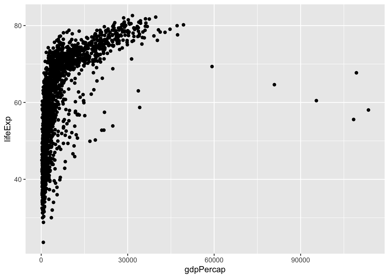

B

ggplot(data = gapminder, 
       mapping = aes(x = gdpPercap, y = lifeExp)) +
  geom_smooth()

`geom_smooth()` using method = 'gam' and formula = 'y ~ s(x, bs = "cs")'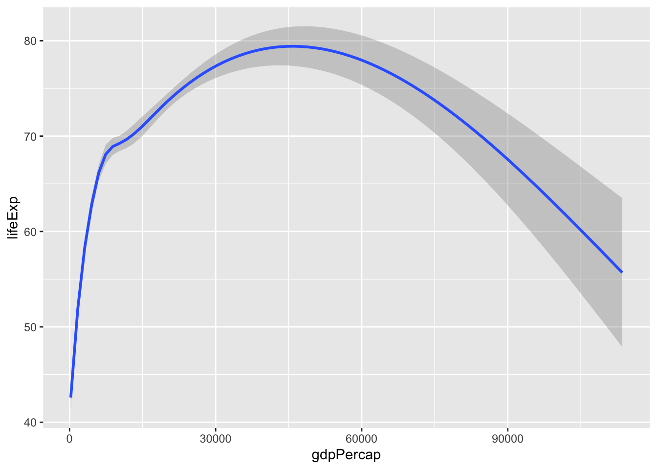

C

ggplot(data = gapminder, 
       mapping = aes(x = gdpPercap, y = lifeExp)) +
  geom_point() + 
  geom_smooth()

`geom_smooth()` using method = 'gam' and formula = 'y ~ s(x, bs = "cs")'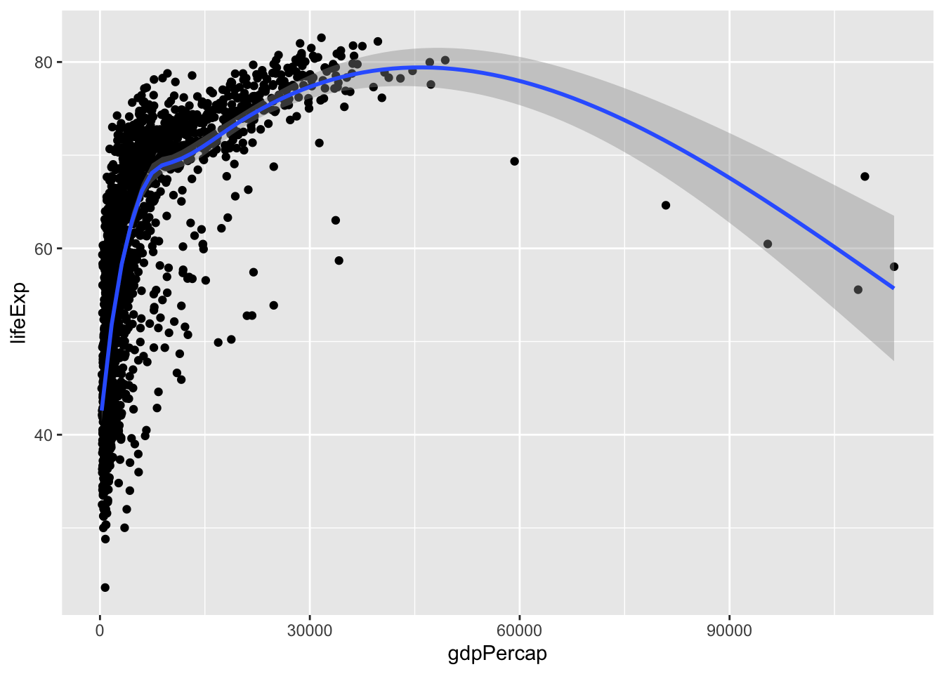

D

ggplot(data = gapminder, 
       mapping = aes(x = gdpPercap, y = lifeExp)) +
  geom_point() + 
  facet_wrap(~ continent)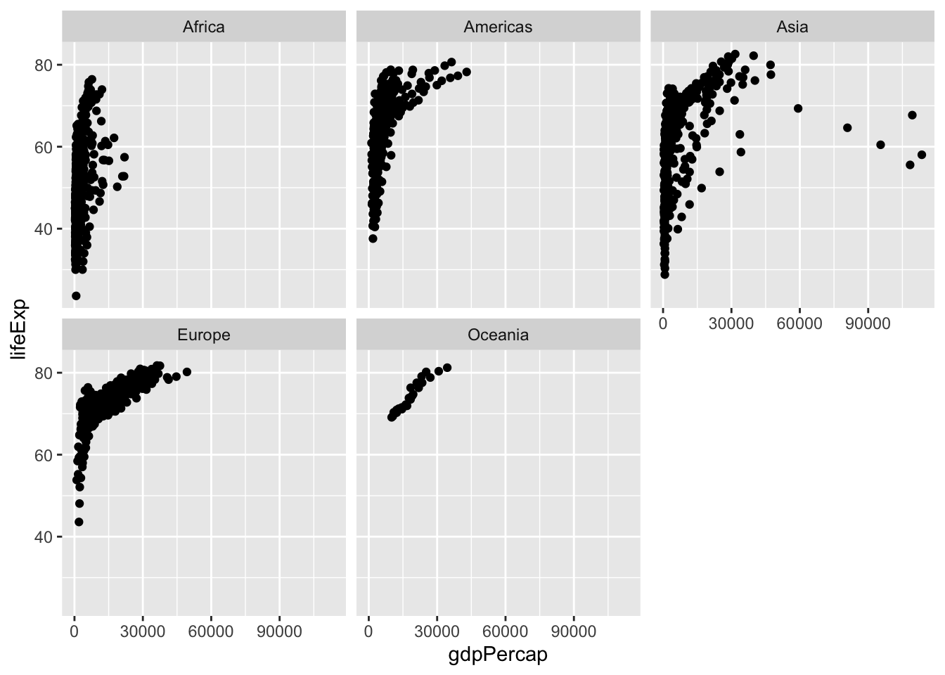

E

ggplot(data = gapminder, 
       mapping = aes(x = lifeExp)) +
  geom_histogram() 

`stat_bin()` using `bins = 30`. Pick better value with `binwidth`.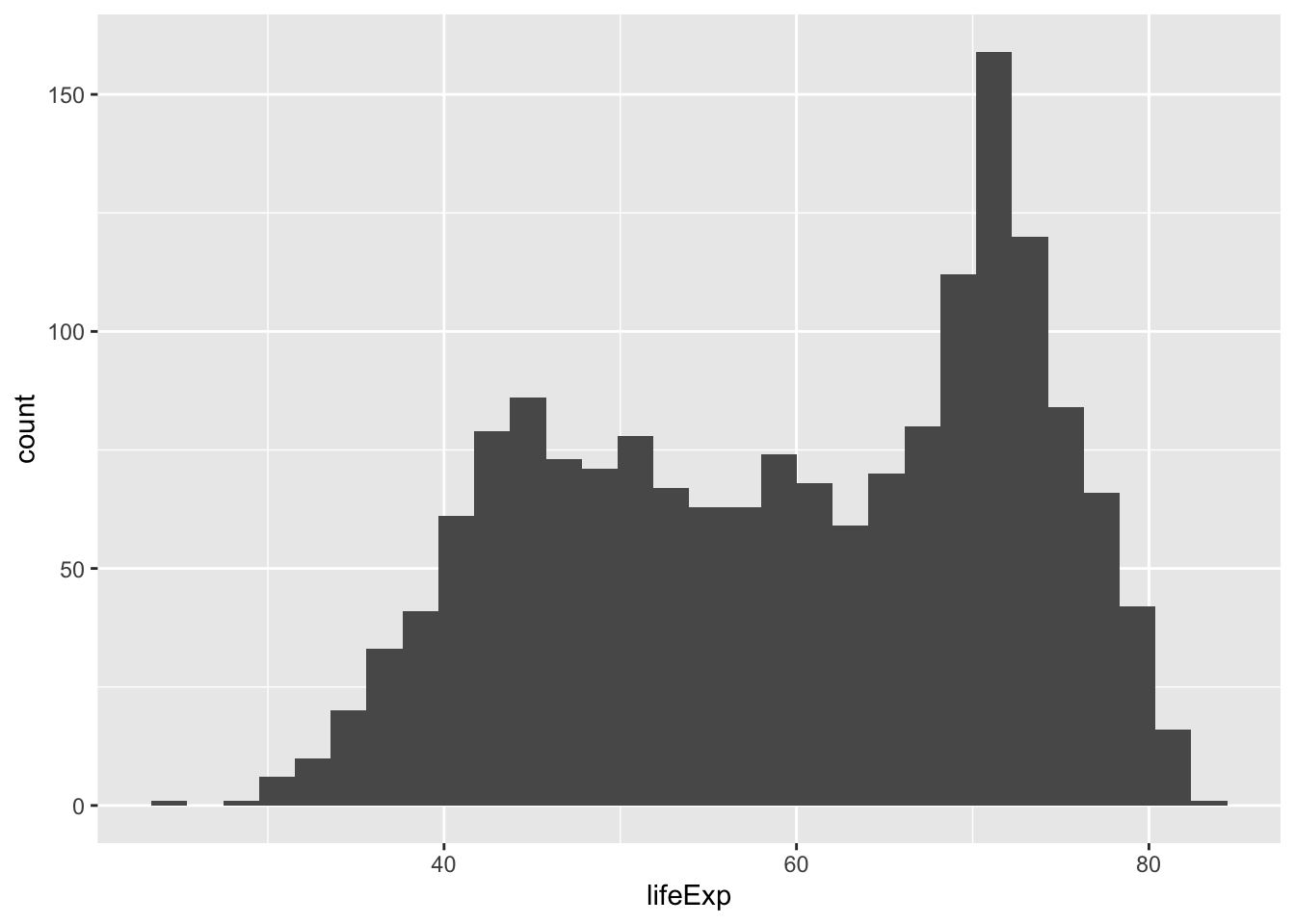

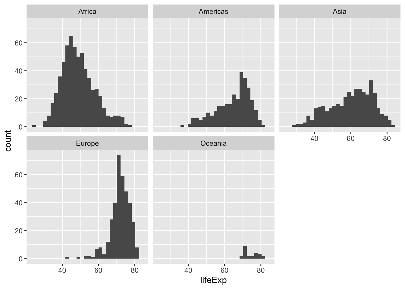
F

ggplot(data = gapminder, 
       mapping = aes(x = lifeExp)) +
  geom_histogram() +
  facet_wrap(~ continent)

`stat_bin()` using `bins = 30`. Pick better value with `binwidth`.