── Conflicts ────────────────────────────────────────── tidyverse_conflicts() ──
✖ dplyr::filter() masks stats::filter()
✖ dplyr::lag()    masks stats::lag()
ℹ Use the conflicted package (<http://conflicted.r-lib.org/>) to force all conflicts to become errors
Core dplyr verbs
Code
gss_sm
# A tibble: 2,867 × 32
    year    id ballot       age childs sibs   degree race  sex   region income16
   <dbl> <dbl> <labelled> <dbl>  <dbl> <labe> <fct>  <fct> <fct> <fct>  <fct>
 1  2016     1 1             47      3 2      Bache… White Male  New E… $170000…
 2  2016     2 2             61      0 3      High … White Male  New E… $50000 …
 3  2016     3 3             72      2 3      Bache… White Male  New E… $75000 …
 4  2016     4 1             43      4 3      High … White Fema… New E… $170000…
 5  2016     5 3             55      2 2      Gradu… White Fema… New E… $170000…
 6  2016     6 2             53      2 2      Junio… White Fema… New E… $60000 …
 7  2016     7 1             50      2 2      High … White Male  New E… $170000…
 8  2016     8 3             23      3 6      High … Other Fema… Middl… $30000 …
 9  2016     9 1             45      3 5      High … Black Male  Middl… $60000 …
10  2016    10 3             71      4 1      Junio… White Male  Middl… $60000 …
# ℹ 2,857 more rows
# ℹ 21 more variables: relig <fct>, marital <fct>, padeg <fct>, madeg <fct>,
#   partyid <fct>, polviews <fct>, happy <fct>, partners <fct>, grass <fct>,
#   zodiac <fct>, pres12 <labelled>, wtssall <dbl>, income_rc <fct>,
#   agegrp <fct>, ageq <fct>, siblings <fct>, kids <fct>, religion <fct>,
#   bigregion <fct>, partners_rc <fct>, obama <dbl>
Select columns
Code
gss_sm |>select(age, degree, bigregion, religion)
# A tibble: 2,867 × 4
     age degree         bigregion religion
   <dbl> <fct>          <fct>     <fct>
 1    47 Bachelor       Northeast None
 2    61 High School    Northeast None
 3    72 Bachelor       Northeast Catholic
 4    43 High School    Northeast Catholic
 5    55 Graduate       Northeast None
 6    53 Junior College Northeast None
 7    50 High School    Northeast None
 8    23 High School    Northeast Catholic
 9    45 High School    Northeast Protestant
10    71 Junior College Northeast None
# ℹ 2,857 more rows
Filter rows
Code
gss_sm |>filter(age >45)
# A tibble: 1,612 × 32
    year    id ballot       age childs sibs   degree race  sex   region income16
   <dbl> <dbl> <labelled> <dbl>  <dbl> <labe> <fct>  <fct> <fct> <fct>  <fct>
 1  2016     1 1             47      3 2      Bache… White Male  New E… $170000…
 2  2016     2 2             61      0 3      High … White Male  New E… $50000 …
 3  2016     3 3             72      2 3      Bache… White Male  New E… $75000 …
 4  2016     5 3             55      2 2      Gradu… White Fema… New E… $170000…
 5  2016     6 2             53      2 2      Junio… White Fema… New E… $60000 …
 6  2016     7 1             50      2 2      High … White Male  New E… $170000…
 7  2016    10 3             71      4 1      Junio… White Male  Middl… $60000 …
 8  2016    12 1             86      4 4      High … White Fema… Middl… under $…
 9  2016    14 3             60      5 6      High … Black Fema… Middl… $12500 …
10  2016    15 2             76      7 0      Lt Hi… White Male  New E… $40000 …
# ℹ 1,602 more rows
# ℹ 21 more variables: relig <fct>, marital <fct>, padeg <fct>, madeg <fct>,
#   partyid <fct>, polviews <fct>, happy <fct>, partners <fct>, grass <fct>,
#   zodiac <fct>, pres12 <labelled>, wtssall <dbl>, income_rc <fct>,
#   agegrp <fct>, ageq <fct>, siblings <fct>, kids <fct>, religion <fct>,
#   bigregion <fct>, partners_rc <fct>, obama <dbl>
Code
gss_sm |>filter(childs >4& race =="White")
# A tibble: 110 × 32
    year    id ballot       age childs sibs   degree race  sex   region income16
   <dbl> <dbl> <labelled> <dbl>  <dbl> <labe> <fct>  <fct> <fct> <fct>  <fct>
 1  2016    15 2             76      7 0      Lt Hi… White Male  New E… $40000 …
 2  2016    17 3             56      6 3      High … White Male  New E… $50000 …
 3  2016    26 2             76      8 7      Lt Hi… White Fema… Middl… $5 000 …
 4  2016   142 3             65      5 2      Junio… White Fema… New E… <NA>
 5  2016   177 1             56      5 3      Bache… White Male  Pacif… $130000…
 6  2016   190 2             51      7 9      Lt Hi… White Fema… Pacif… $15000 …
 7  2016   216 3             77      8 9      High … White Male  Pacif… $60000 …
 8  2016   351 3             52      5 4      High … White Fema… E. No… $35000 …
 9  2016   365 1             51      5 5      Gradu… White Male  South… $170000…
10  2016   379 3             NA      7 2      High … White Male  South… $170000…
# ℹ 100 more rows
# ℹ 21 more variables: relig <fct>, marital <fct>, padeg <fct>, madeg <fct>,
#   partyid <fct>, polviews <fct>, happy <fct>, partners <fct>, grass <fct>,
#   zodiac <fct>, pres12 <labelled>, wtssall <dbl>, income_rc <fct>,
#   agegrp <fct>, ageq <fct>, siblings <fct>, kids <fct>, religion <fct>,
#   bigregion <fct>, partners_rc <fct>, obama <dbl>
Logically Group with group_by()
Code
gss_sm |>group_by(bigregion)
# A tibble: 2,867 × 32
# Groups:   bigregion [4]
    year    id ballot       age childs sibs   degree race  sex   region income16
   <dbl> <dbl> <labelled> <dbl>  <dbl> <labe> <fct>  <fct> <fct> <fct>  <fct>
 1  2016     1 1             47      3 2      Bache… White Male  New E… $170000…
 2  2016     2 2             61      0 3      High … White Male  New E… $50000 …
 3  2016     3 3             72      2 3      Bache… White Male  New E… $75000 …
 4  2016     4 1             43      4 3      High … White Fema… New E… $170000…
 5  2016     5 3             55      2 2      Gradu… White Fema… New E… $170000…
 6  2016     6 2             53      2 2      Junio… White Fema… New E… $60000 …
 7  2016     7 1             50      2 2      High … White Male  New E… $170000…
 8  2016     8 3             23      3 6      High … Other Fema… Middl… $30000 …
 9  2016     9 1             45      3 5      High … Black Male  Middl… $60000 …
10  2016    10 3             71      4 1      Junio… White Male  Middl… $60000 …
# ℹ 2,857 more rows
# ℹ 21 more variables: relig <fct>, marital <fct>, padeg <fct>, madeg <fct>,
#   partyid <fct>, polviews <fct>, happy <fct>, partners <fct>, grass <fct>,
#   zodiac <fct>, pres12 <labelled>, wtssall <dbl>, income_rc <fct>,
#   agegrp <fct>, ageq <fct>, siblings <fct>, kids <fct>, religion <fct>,
#   bigregion <fct>, partners_rc <fct>, obama <dbl>
The \(x) introduces an anonymous function or lambda. The x means “the thing” or “the thing we’re doing something to right now”, and what follows it is some operation we perform on the thing.
# A tibble: 238 × 21
   country   year       donors   pop pop_dens   gdp gdp_lag health health_lag
   <chr>     <date>      <dbl> <dbl>    <dbl> <int>   <int>  <dbl>      <dbl>
 1 Australia NA          NA    17065        0 16774   16591   1300       1224
 2 Australia 1991-01-01  12.1  17284        0 17171   16774   1379       1300
 3 Australia 1992-01-01  12.4  17495        0 17914   17171   1455       1379
 4 Australia 1993-01-01  12.5  17667        0 18883   17914   1540       1455
 5 Australia 1994-01-01  10.2  17855        0 19849   18883   1626       1540
 6 Australia 1995-01-01  10.2  18072        0 21079   19849   1737       1626
 7 Australia 1996-01-01  10.6  18311        0 21923   21079   1846       1737
 8 Australia 1997-01-01  10.3  18518        0 22961   21923   1948       1846
 9 Australia 1998-01-01  10.5  18711        0 24148   22961   2077       1948
10 Australia 1999-01-01   8.67 18926        0 25445   24148   2231       2077
# ℹ 228 more rows
# ℹ 12 more variables: pubhealth <dbl>, roads <dbl>, cerebvas <int>,
#   assault <int>, external <int>, txp_pop <dbl>, world <chr>, opt <chr>,
#   consent_law <chr>, consent_practice <chr>, consistent <chr>, ccode <chr>
The function can be a named one, or you can write something yourself:
Code
organdata |>mutate(across(starts_with("pop"), \(x) x /100))
# A tibble: 238 × 21
   country   year       donors   pop pop_dens   gdp gdp_lag health health_lag
   <chr>     <date>      <dbl> <dbl>    <dbl> <int>   <int>  <dbl>      <dbl>
 1 Australia NA          NA     171.  0.00220 16774   16591   1300       1224
 2 Australia 1991-01-01  12.1   173.  0.00223 17171   16774   1379       1300
 3 Australia 1992-01-01  12.4   175.  0.00226 17914   17171   1455       1379
 4 Australia 1993-01-01  12.5   177.  0.00228 18883   17914   1540       1455
 5 Australia 1994-01-01  10.2   179.  0.00231 19849   18883   1626       1540
 6 Australia 1995-01-01  10.2   181.  0.00233 21079   19849   1737       1626
 7 Australia 1996-01-01  10.6   183.  0.00237 21923   21079   1846       1737
 8 Australia 1997-01-01  10.3   185.  0.00239 22961   21923   1948       1846
 9 Australia 1998-01-01  10.5   187.  0.00242 24148   22961   2077       1948
10 Australia 1999-01-01   8.67  189.  0.00244 25445   24148   2231       2077
# ℹ 228 more rows
# ℹ 12 more variables: pubhealth <dbl>, roads <dbl>, cerebvas <int>,
#   assault <int>, external <int>, txp_pop <dbl>, world <chr>, opt <chr>,
#   consent_law <chr>, consent_practice <chr>, consistent <chr>, ccode <chr>
You can use where() with select() as well, when you are just subsetting by column but not yet doing anything across the columns:
Code
organdata |>select(where(is.character))
# A tibble: 238 × 7
   country   world   opt   consent_law consent_practice consistent ccode
   <chr>     <chr>   <chr> <chr>       <chr>            <chr>      <chr>
 1 Australia Liberal In    Informed    Informed         Yes        Oz
 2 Australia Liberal In    Informed    Informed         Yes        Oz
 3 Australia Liberal In    Informed    Informed         Yes        Oz
 4 Australia Liberal In    Informed    Informed         Yes        Oz
 5 Australia Liberal In    Informed    Informed         Yes        Oz
 6 Australia Liberal In    Informed    Informed         Yes        Oz
 7 Australia Liberal In    Informed    Informed         Yes        Oz
 8 Australia Liberal In    Informed    Informed         Yes        Oz
 9 Australia Liberal In    Informed    Informed         Yes        Oz
10 Australia Liberal In    Informed    Informed         Yes        Oz
# ℹ 228 more rows
If you use a function like mean() or sd() or n() with mutate() instead of summarize() it will work too. The difference is that a column will be added with the value repeated for all group members. This can be useful when you want e.g. to make a denominator for some calculation later. Remember, mutate() adds or changes columns but never changes the number of rows in the table, whereas summarize() will usually output a table with fewer rows than the one you give it.
Code
## Country-year data, 238 rows altogether,## with yearly data for 17 countries.organdata |>select(country, donors)
# A tibble: 238 × 2
   country   donors
   <chr>      <dbl>
 1 Australia  NA
 2 Australia  12.1
 3 Australia  12.4
 4 Australia  12.5
 5 Australia  10.2
 6 Australia  10.2
 7 Australia  10.6
 8 Australia  10.3
 9 Australia  10.5
10 Australia   8.67
# ℹ 228 more rows
Code
## Summarize gets you one row per countryorgandata |>select(country, donors) |>group_by(country) |>summarize(donors_mean =mean(donors, na.rm =TRUE))
# A tibble: 17 × 2
   country        donors_mean
   <chr>                <dbl>
 1 Australia             10.6
 2 Austria               23.5
 3 Belgium               21.9
 4 Canada                14.0
 5 Denmark               13.1
 6 Finland               18.4
 7 France                16.8
 8 Germany               13.0
 9 Ireland               19.8
10 Italy                 11.1
11 Netherlands           13.7
12 Norway                15.4
13 Spain                 28.1
14 Sweden                13.1
15 Switzerland           14.2
16 United Kingdom        13.5
17 United States         20.0
Code
## Mutate adds each country's donor mean ## to the 238 observationstmp <- organdata |>select(country, donors) |>group_by(country) |>mutate(donors_mean =mean(donors, na.rm =TRUE))# First few rows of 238head(tmp)
# A tibble: 6 × 3
# Groups:   country [1]
  country   donors donors_mean
  <chr>      <dbl>       <dbl>
1 Australia   NA          10.6
2 Australia   12.1        10.6
3 Australia   12.4        10.6
4 Australia   12.5        10.6
5 Australia   10.2        10.6
6 Australia   10.2        10.6
Code
# Last few rows of 238tail(tmp)
# A tibble: 6 × 3
# Groups:   country [1]
  country       donors donors_mean
  <chr>          <dbl>       <dbl>
1 United States   21          20.0
2 United States   20.9        20.0
3 United States   21.2        20.0
4 United States   21.3        20.0
5 United States   21.5        20.0
6 United States   NA          20.0
Graph your summarized tables
Code
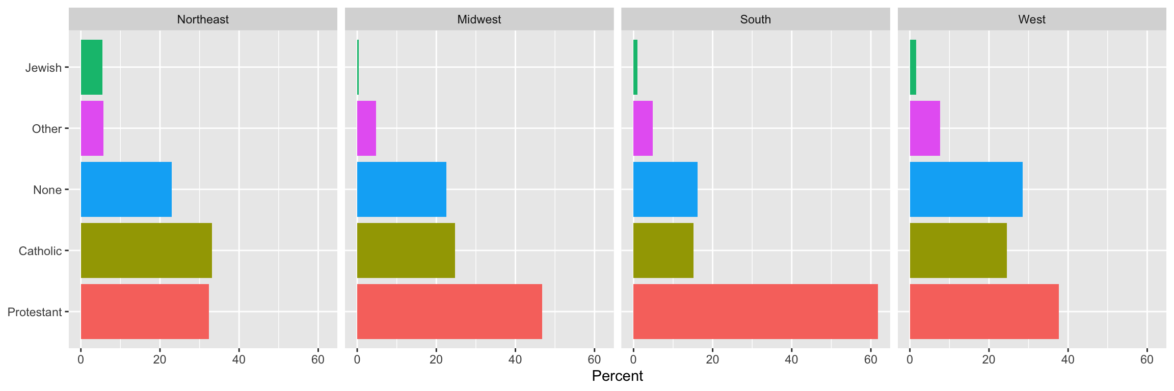
gss_sm |>group_by(bigregion, religion) |>tally() |>mutate(pct =round((n/sum(n))*100, 1)) |>drop_na() |>ggplot(mapping =aes(x = pct, y =reorder(religion, -pct), fill = religion)) +geom_col() +labs(x ="Percent", y =NULL) +guides(fill ="none") +facet_wrap(~ bigregion, nrow =1)
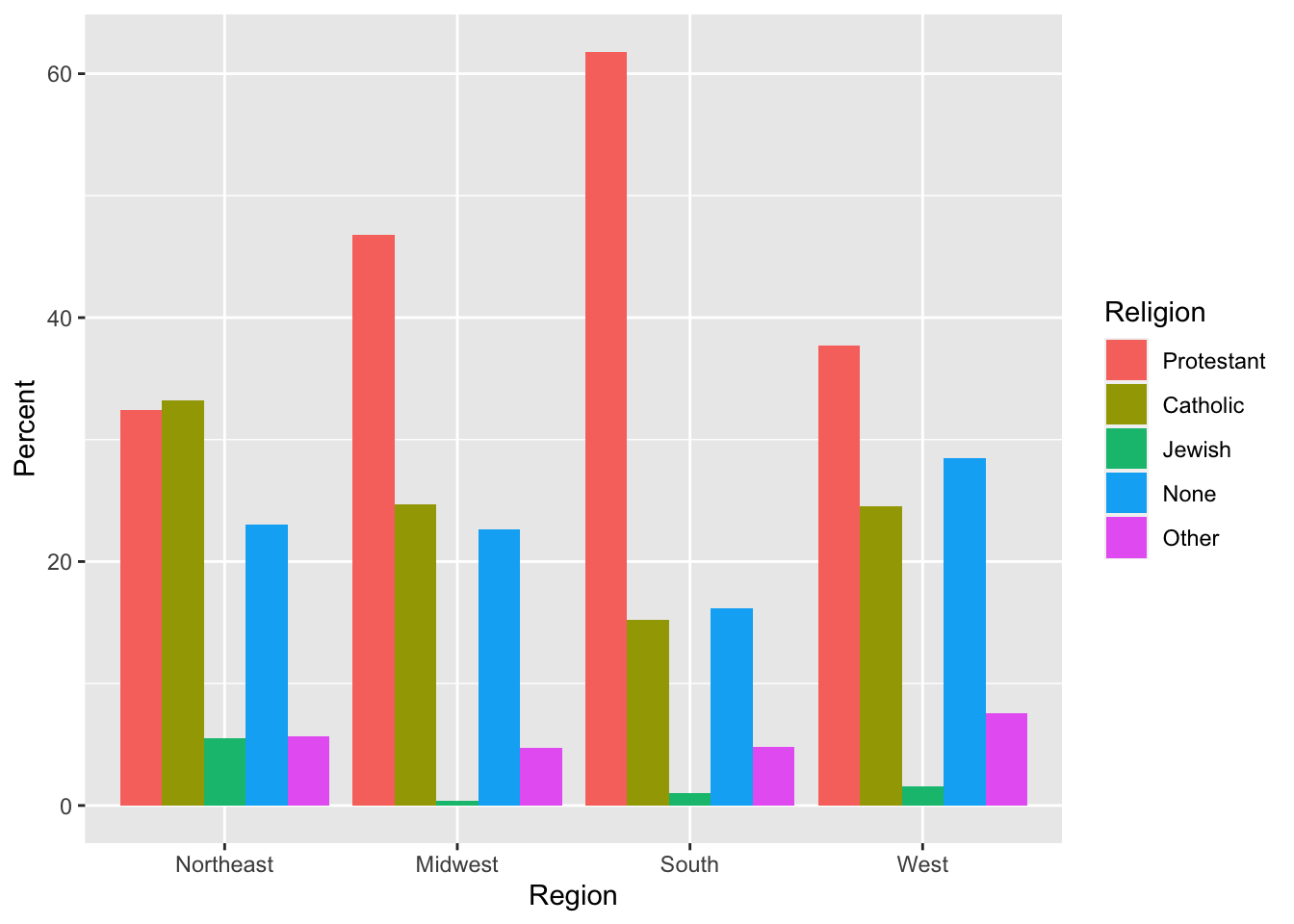
p <-ggplot(data = rel_by_region, mapping =aes(x = bigregion, y = pct, fill = religion))p_out <- p +geom_col(position ="dodge") +labs(x ="Region",y ="Percent", fill ="Religion") p_out
Experiment with facets:
Code
p <-ggplot(data = rel_by_region, mapping =aes(x = pct, y =reorder(religion, -pct), fill = religion))p_out_facet <- p +geom_col() +guides(fill ="none") +facet_wrap(~ bigregion, nrow =1) +labs(x ="Percent",y =NULL) p_out_facet
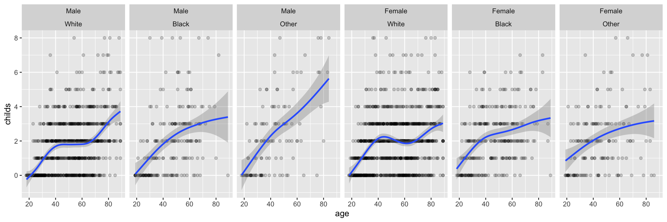
Multi-way facets
Code
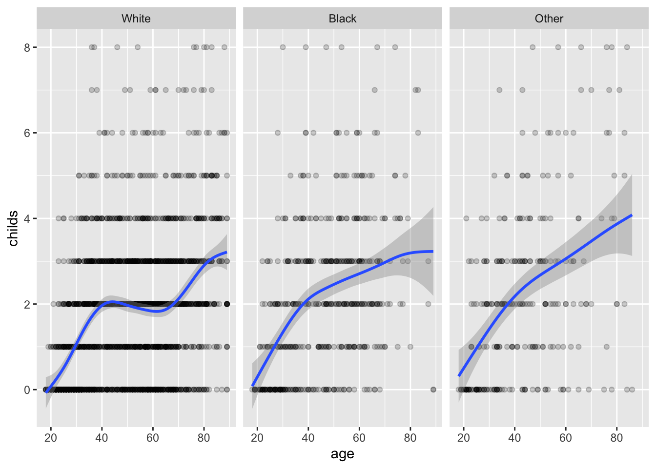
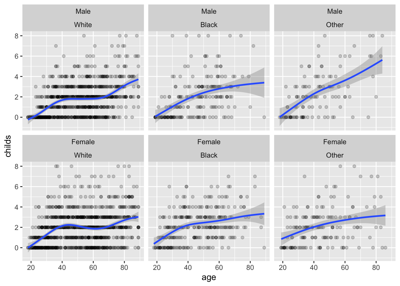
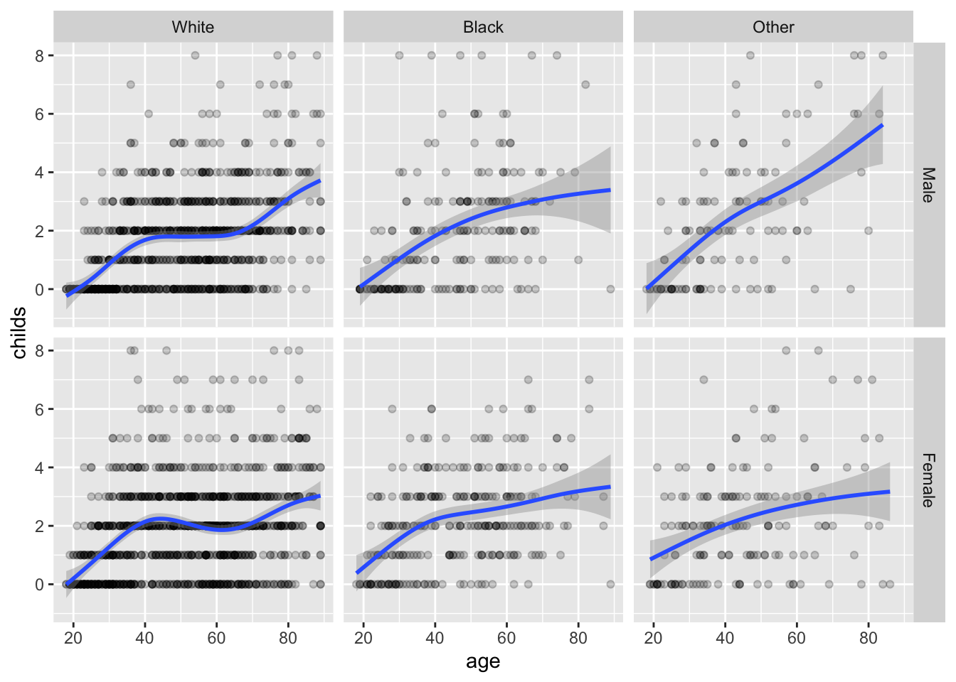
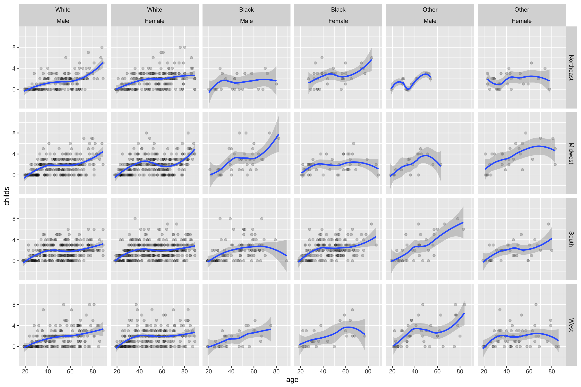
p <-ggplot(data = gss_sm,mapping =aes(x = age, y = childs))p +geom_point(alpha =0.2) +geom_smooth() +facet_wrap(~ race)
`geom_smooth()` using method = 'gam' and formula = 'y ~ s(x, bs = "cs")'
---title: "Example 05: Working with `dplyr`"---## Setup```{r}library(here) # manage file pathslibrary(socviz) # data and some useful functionslibrary(tidyverse) # your friend and mine```## Core `dplyr` verbs```{r}gss_sm ```### Select columns```{r}gss_sm |>select(age, degree, bigregion, religion)```### Filter rows```{r}gss_sm |>filter(age >45)``````{r}gss_sm |>filter(childs >4& race =="White")```## Logically Group with `group_by()````{r}gss_sm |>group_by(bigregion)```### Summarize groups with `summarize()````{r}gss_sm |>group_by(bigregion) |>summarize(total =n()) ```### Multi-way groupings```{r}gss_sm |>group_by(bigregion, religion) |>summarize(total =n()) ```### Add columns with `mutate()````{r}gss_sm |>group_by(bigregion, religion) |>summarize(total =n()) |>mutate(freq = total /sum(total),pct =round((freq*100), 1))```## Tally and Count- Do it yourself:```{r}gss_sm |>group_by(bigregion, religion) |>summarize(n =n()) ```- Use `tally()`:```{r}gss_sm |>group_by(bigregion, religion) |>tally() ```- Use `count()`:```{r}gss_sm |>count(bigregion, religion) ```Pay attention to how grouping works in these summaries.## Check your work```{r}rel_by_region <- gss_sm |>count(bigregion, religion) |>mutate(pct =round((n/sum(n))*100, 1)) rel_by_region```- Each region should sum to ~100```{r}rel_by_region |>group_by(bigregion) |>summarize(total =sum(pct)) ```- Grouping has caught us out. Try again.```{r}rel_by_region <- gss_sm |>count(bigregion, religion) |>mutate(pct =round((n/sum(n))*100, 1)) rel_by_region```## Summarize returns one tibble row per group```{r}gss_sm |>group_by(bigregion) |>tally()```When you have 2 or n-way groups the calculation is done from the inside out, on the innermost group. ```{r}# 4 regions, 6 religion = 24 groupsgss_sm |>group_by(bigregion, religion) |>tally()```## Summarize many variablesThe inefficient way:```{r}organdata |>group_by(consent_law, country) |>summarize(donors_mean=mean(donors, na.rm =TRUE),donors_sd =sd(donors, na.rm =TRUE),gdp_mean =mean(gdp, na.rm =TRUE),gdp_sd =sd(gdp, na.rm =TRUE),health_mean =mean(health, na.rm =TRUE),roads_mean =mean(roads, na.rm =TRUE),cerebvas_mean =mean(cerebvas, na.rm =TRUE))```## Use `across()` and `where()` insteadBetter:```{r}organdata |>group_by(consent_law, country) |>summarize(across(where(is.numeric),list(mean = \(x) mean(x, na.rm =TRUE), sd = \(x) sd(x, na.rm =TRUE))))```The `\(x)` introduces an _anonymous function_ or _lambda_. The `x` means "the thing" or "the thing we're doing something to right now", and what follows it is some operation we perform on the thing. Optionally drop any remaning groups:```{r}organdata |>group_by(consent_law, country) |>summarize(across(where(is.numeric),list(mean = \(x) mean(x, na.rm =TRUE), sd = \(x) sd(x, na.rm =TRUE))),.groups ="drop")```- The `across()` function is used _inside_ `summarize()` and `mutate()` to do something across some subset of columns. - Inside `across()`, use `where()` to choose columns, and then apply a function to each of them. ```{r}organdata |>mutate(across(where(is.numeric), round))```You can also use various "tidy selectors", like this:```{r}organdata |>mutate(across(starts_with("pop"), round))```The function can be a named one, or you can write something yourself:```{r}organdata |>mutate(across(starts_with("pop"), \(x) x /100))```You can use `where()` with `select()` as well, when you are just subsetting by column but not yet doing anything across the columns:```{r}organdata |>select(where(is.character))``````{r}organdata |>select(starts_with("gdp"))``````{r}organdata |>select(contains("health"))```## Reminder: the `%in%` operatorThis is a useful way to restrict selections of either columns, with `select()`, or especially rows, with (`filter`):```{r}organdata |>filter(country %in%c("Ireland", "Italy", "Spain"))```## All this applies to `mutate()` as wellIf you use a function like `mean()` or `sd()` or `n()` with `mutate()` instead of `summarize()` it will work too. The difference is that a column will be added with the value repeated for all group members. This can be useful when you want e.g. to make a denominator for some calculation later. Remember, `mutate()` adds or changes columns but never changes the number of rows in the table, whereas `summarize()` will usually output a table with fewer rows than the one you give it.```{r}## Country-year data, 238 rows altogether,## with yearly data for 17 countries.organdata |>select(country, donors)``````{r}## Summarize gets you one row per countryorgandata |>select(country, donors) |>group_by(country) |>summarize(donors_mean =mean(donors, na.rm =TRUE))``````{r}## Mutate adds each country's donor mean ## to the 238 observationstmp <- organdata |>select(country, donors) |>group_by(country) |>mutate(donors_mean =mean(donors, na.rm =TRUE))# First few rows of 238head(tmp)# Last few rows of 238tail(tmp)```## Graph your summarized tables```{r, fig.width=12, fig.height = 4}gss_sm |> group_by(bigregion, religion) |> tally() |> mutate(pct = round((n/sum(n))*100, 1)) |> drop_na() |> ggplot(mapping = aes(x = pct, y = reorder(religion, -pct), fill = religion)) + geom_col() + labs(x = "Percent", y = NULL) + guides(fill = "none") + facet_wrap(~ bigregion, nrow = 1)``````{r}rel_by_region <- gss_sm |>group_by(bigregion, religion) |>tally() |>mutate(pct =round((n/sum(n))*100, 1)) |>drop_na()head(rel_by_region)``````{r}p <-ggplot(data = rel_by_region, mapping =aes(x = bigregion, y = pct, fill = religion))p_out <- p +geom_col(position ="dodge") +labs(x ="Region",y ="Percent", fill ="Religion") p_out```Experiment with facets:```{r, fig.width=12, fig.height=4}p <- ggplot(data = rel_by_region, mapping = aes(x = pct, y = reorder(religion, -pct), fill = religion))p_out_facet <- p + geom_col() + guides(fill = "none") + facet_wrap(~ bigregion, nrow = 1) + labs(x = "Percent", y = NULL) p_out_facet```## Multi-way facets```{r}p <-ggplot(data = gss_sm,mapping =aes(x = age, y = childs))p +geom_point(alpha =0.2) +geom_smooth() +facet_wrap(~ race)``````{r}p <-ggplot(data = gss_sm,mapping =aes(x = age, y = childs))p +geom_point(alpha =0.2) +geom_smooth() +facet_wrap(~ sex + race) ``````{r, fig.width=12, fig.height=4}p <- ggplot(data = gss_sm, mapping = aes(x = age, y = childs))p + geom_point(alpha = 0.2) + geom_smooth() + facet_wrap(~ sex + race, nrow = 1) ```### `facet_wrap()` vs `facet_grid()````{r}p +geom_point(alpha =0.2) +geom_smooth() +facet_grid(sex ~ race) ``````{r, fig.width=12, fig.height=8}p_out <- p + geom_point(alpha = 0.2) + geom_smooth() + facet_grid(bigregion ~ race + sex) p_out```